1. CHAPTER 7
Probability and Samples:
Distribution of Sample Means

2. Probability and Samples: Chap 7
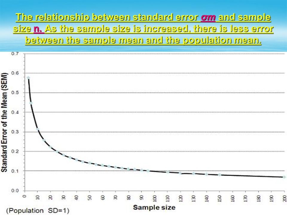
Sampling Error The amount of error between a sample statistic (M) and population parameter (µ). Distribution of Sample Means: is the collection of sample means for all the possible random samples of a particular size (n) that can be obtained from a population.

4. Sampling Distribution
Sampling Distribution is a distribution of statistics obtained by selecting all the possible samples of a specific size from a population. Ex. Every distribution has a mean and standard deviation. The mean of all sample means is called Sampling Distribution. The mean of all standard deviations is called Standard Error of Mean (σM)

5. Expected Value of M
The mean of the distribution of (M) sample means (statistics) is equal to the mean of the Population of scores (µ) and is called the Expected Value of M M= µ And, the average standard deviation (S) for all of these means is called Standard Error of Mean, σM. It provides a measure of how much distance is expected on average between a sample mean (M) and the population mean (µ)

6. The Law of Large Numbers
The Law of Large Numbers states that the larger the sample size (n), the more probable it is that the sample mean (M) will be close to the population mean (µ) n≈ N

7. Probability and Samples
The Central Limit Theorem:
Describes the distribution of sample means by identifying 3 basic characteristics that describe any distribution: 1. The shape of the distribution of sample mean has 2 conditions 1a. The population from which the samples are selected is normal distribution. 1b. The number of scores (n) in each sample is relatively large
(30 or more) The larger the n the shape of the distribution tends to be more normal.

8. The Central Limit Theorem:
2. Central Tendency: Stats that the mean of the distribution of sample means M is equal to the population mean µ and is called the expected value of M. M= µ
3. Variability: or the standard error of mean σM.
The standard deviation of the distribution of sample means is called the standard error of mean σM.
It measures the standard amount of difference one should expect between M and µ simply due to chance.

9. Computations/ Calculations or Collect Data and Compute Sample Statistics Z Score for Research

10. Computations/ Calculations or Collect Data and Compute Sample Statistics Z Score for Research

11. Computations/ Calculations or Collect Data and Compute Sample Statistics Z Score for Research

12. Computations/ Calculations or Collect Data and Compute Sample Statistics
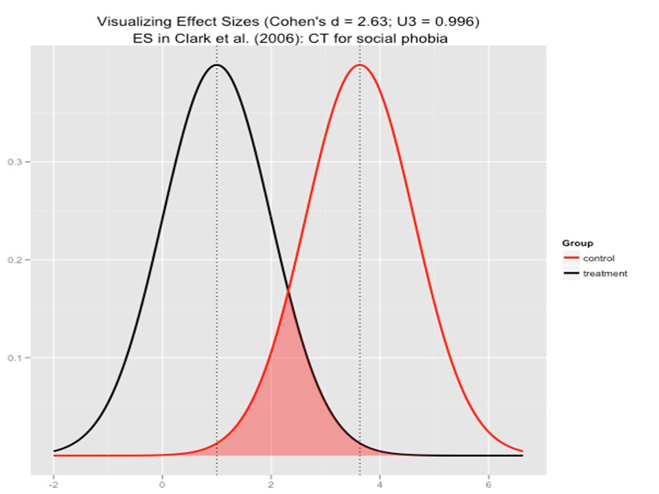
d=Effect Size/Cohn d
Is the difference between the means in a treatment condition.
It means that the result from a research study is not just by chance alone

14. Computations/ Calculations or Collect Data and Compute Sample Statistics d=Effect Size

16. Problem 1
The population of scores on the SAT forms a normal distribution with µ=500 and σ=100. If you take a random sample of n=25 students, what is the probability (%) that the sample mean will be greater than 540. M=540?
First calculate the Z Score then, look for proportion and convert into percentage.

17. Problem 2
Once again, the distribution of SAT forms a normal distribution with a mean of µ=500 and σ=100. For this example we are going to determine what kind of sample mean (M) is likely to be obtained as the average SAT score for a random sample of n=25 students. Specifically, we will determine the exact range of values that is expected for the sample mean 80% of the time.

18. CHAPTER 8
Hypothesis Testing

19. Chap 8Hypothesis Testing
Hypothesis : Statement such as “The relationship between IQ and GPA. Topic of a research.
Hypothesis Test: Is a statistical method that uses sample data to evaluate a hypothesis about a population.
The statistics used to Test a hypothesis is called “Test Statistic” i.e., Z, t, r, F, etc.

20. Hypothesis Testing
The Logic of Hypothesis: If the sample mean is consistent with the prediction we conclude that the hypothesis is reasonable but, if there is a big discrepancy we decide that hypothesis is not reasonable.
Ex. Registered Voters are Smarter than Average People.

21. Role of Statistics in Research

22. Steps in Hypothesis-Testing Step 1: State The Hypotheses
H0=Null Hypothesis
H1 :Alternative or Researcher Hypothesis

23. Steps in Hypothesis-Testing Step 1: State The Hypotheses
H0 : µ ≤ 100 average
H1 : µ > 100 average
Statistics:
Because the Population mean or µ is known the statistic of choice is
z-Score

24. Hypothesis Testing Step 2: Locate the Critical Region(s) or Set the Criteria for a Decision

25. Directional Hypothesis Test

26. None-directional Hypothesis Test

27. Hypothesis Testing Step 3: Computations/ Calculations or Collect Data and Compute Sample Statistics

28. Hypothesis Testing Step 4: Make a Decision

29. Hypothesis Testing Step 4: Make a Decision

30. Uncertainty and Errors in Hypothesis Testing
Type I Error
Type II Error see next slide
True H0
False H0
Reject
Type I Error α
Correct Decision
Power=1-β
Retain
Type II error β

31. True H0 False H0 True State of the World Reject Type I Error α
Correct Decision
Power=1-β
Retain
Type II error β

32. Power
Power:
The power of a statistical test is the probability that the test will correctly reject a false null hypothesis.
That is, power is the probability that the test will identify a treatment effect if one really exists.

33. The α level or the level of significance:
The α level for a hypothesis test is the probability that the test will lead to a Type I error.
That is, the alpha level determines the probability of obtaining sample data in the critical region even though the null hypothesis is true.

34. The α level or the level of significance:
It is a probability value which is used to define the concept of “highly unlikely” in a hypothesis test.

35. The Critical Region
Is composed of the extreme sample values that are highly unlikely (as defined by the α level or the level of significance) to be obtained if the null hypothesis is true.
If sample data fall in the critical region, the null hypothesis is rejected.

36. Computations/ Calculations or Collect Data and Compute Sample Statistics
d=Effect Size/Cohn d
It is the difference between the means in a treatment condition.
It means that the result from a research study is not just by chance alone

37. Effect Size=Cohn’s d
Effect Size=Cohn’s d= Result from the research study is bigger than what we expected to be just by chance alone.

39. Cohn’s d=Effect Size

40. Evaluation of Cohn’s d Effect Size with Cohn’s d
Magnitude of d
Evaluation of Effect Size
d≈0.2
Small Effect Size
d≈0.5
Medium Effect Size
d≈0.8
Large Effect Size

41. Problems
Researchers have noted a decline in cognitive functioning as people age (Bartus, 1990) However, the results from other research suggest that the antioxidants in foods such as blueberries can reduce and even reverse these age-related declines, at least in laboratory rats (Joseph, Shukitt-Hale, Denisova, et al., 1999). Based on these results one might theorize that the same antioxidants might also benefit elderly humans. Suppose a researcher is interested in testing this theory. Next slide

42. Problems
Standardized neuropsychological tests such as the Wisconsin Card Sorting Test WCST can be use to measure conceptual thinking ability and mental flexibility (Heaton, Chelune, Talley, Kay, & Kurtiss, 1993). Performance on this type of test declines gradually with age. Suppose our researcher selects a test for which adults older than 65 have an average score of μ=80 with a standard deviation of σ=20. The distribution of test score is approximately normal. The researcher plan is to obtain a sample of n=25 adults who are older than 65, and give each participants a daily dose of blueberry supplement that is very high in antioxidants. After taking the supplement for 6 months

43. Problems
The participants were given the neuropsychological tests to measure their level of cognitive function. M=92, 2 tailed,
α = 0.05
The hypothesis is that the blubbery supplement does appear to have an effect on cognitive functioning.
Step 1
H0 : μ with supplement = 80
H1 : μ with supplement ≠ 80

44. None-directional Hypothesis Test

45. Problems M=92, one tailed, α = 0.05
If the hypothesis stated that the consumption of blubbery supplement will increase the cognitive functioning (test scores) then,
Step 1
H0 : μ ≤ 80
H1 : μ > 80

46. Directional Hypothesis Test

47. Problems M=92, one tailed, α = 0.05
If the hypothesis stated that the consumption of blubbery supplement will decrease the cognitive functioning (test scores) then,
Step 1
H0 : μ ≥ 80
H1 : μ < 80

48. Directional Hypothesis Test

49. Problems
Alcohol appears to be involve in a variety of birth defects, including low birth weight and retarded growth. A researcher would like to investigate the effect of prenatal alcohol on birth weight . A random sample of n=16 pregnant rats is obtained. The mother rats are given daily dose of alcohol. At birth, one pop is selected from each litter to produce a sample of n=16 newborn rats. The average weight for the sample is M=16 grams.

50. The researcher would like to compare the sample with the general population of rats. It is known that regular new born rats have an average weight of μ=18 grams. The distribution of weight is normal with σ=4, set α=0.01, and we use a 2 tailed test consequently, on each tail and the critical value for Z= Step 1
H0 : μ alcohol exposure = 18 grams
H1 : μ alcohol exposure ≠ 18 grams
Problems

51. Degrees of Freedom df=n-1

52. Standard Deviation of Sample