1. From SAT to SMT A Tutorial Nikolaj Bjørner Microsoft Research Dagstuhl April 23, 2015

2. Plan SMT in a nutshell SMT solving walkthrough by example Selected Theory solvers – Equalities – Arrays – Arithmetic Combining Solvers

3. Is formula  satisfiable modulo theory T ? SMT solvers have specialized algorithms for T Satisfiability Modulo Theories (SMT)

4. ArithmeticArithmetic Array Theory Uninterpreted Functions Satisfiability Modulo Theories (SMT)

5. SAT Theory Solvers SMT SMT: Basic Architecture Equality + UF Arithmetic Bit-vectors … Case Analysis

6. SAT + Theory solvers Basic Idea x  0, y = x + 1, (y > 2  y < 1) p 1, p 2, (p 3  p 4 ) Abstract (aka “naming” atoms) p 1  (x  0), p 2  (y = x + 1), p 3  (y > 2), p 4  (y < 1)

7. SAT + Theory solvers Basic Idea x  0, y = x + 1, (y > 2  y < 1) p 1, p 2, (p 3  p 4 ) Abstract (aka “naming” atoms) p 1  (x  0), p 2  (y = x + 1), p 3  (y > 2), p 4  (y < 1) SAT Solver SAT Solver

8. SAT + Theory solvers Basic Idea x  0, y = x + 1, (y > 2  y < 1) p 1, p 2, (p 3  p 4 ) Abstract (aka “naming” atoms) p 1  (x  0), p 2  (y = x + 1), p 3  (y > 2), p 4  (y < 1) SAT Solver SAT Solver Assignment p 1, p 2,  p 3, p 4

9. SAT + Theory solvers Basic Idea x  0, y = x + 1, (y > 2  y < 1) p 1, p 2, (p 3  p 4 ) Abstract (aka “naming” atoms) p 1  (x  0), p 2  (y = x + 1), p 3  (y > 2), p 4  (y < 1) SAT Solver SAT Solver Assignment p 1, p 2,  p 3, p 4 x  0, y = x + 1,  (y > 2), y < 1

10. SAT + Theory solvers Basic Idea x  0, y = x + 1, (y > 2  y < 1) p 1, p 2, (p 3  p 4 ) Abstract (aka “naming” atoms) p 1  (x  0), p 2  (y = x + 1), p 3  (y > 2), p 4  (y < 1) SAT Solver SAT Solver Assignment p 1, p 2,  p 3, p 4 x  0, y = x + 1,  (y > 2), y < 1 Theory Solver Theory Solver Unsatisfiable x  0, y = x + 1, y < 1

11. SAT + Theory solvers Basic Idea x  0, y = x + 1, (y > 2  y < 1) p 1, p 2, (p 3  p 4 ) Abstract (aka “naming” atoms) p 1  (x  0), p 2  (y = x + 1), p 3  (y > 2), p 4  (y < 1) SAT Solver SAT Solver Assignment p 1, p 2,  p 3, p 4 x  0, y = x + 1,  (y > 2), y < 1 Theory Solver Theory Solver Unsatisfiable x  0, y = x + 1, y < 1 New Lemma  p 1  p 2  p 4

12. SAT + Theory solvers Theory Solver Theory Solver Unsatisfiable x  0, y = x + 1, y < 1 New Lemma  p 1  p 2  p 4 AKA Theory conflict AKA Theory conflict

13. SAT/SMT SOLVING USING DPLL(T)/CDCL

14. Proofs Conflict Clauses Proofs Models literal assignments Models Conflict Resolution BackjumpBackjump PropagatePropagate Mile High: Modern SAT/SMT search

15. Core Engine in Z3: Modern DPLL/CDCL Initialize Decide Propagate Sat Conflict Learn Unsat Backjump Resolve Forget Restart [Nieuwenhuis, Oliveras, Tinelli J.ACM 06] customized Model Proof Conflict Resolution

16. DPLL(T) solver interaction

17. MCSat [Jojanovich, de Moura] (Cotton, McMillan, Nieuwenhuis, Voronkov,,…) Search – Trail: values guessed for sub-terms – Propagate values, derive consequences – Conflict resolution: Detect, backjump, learn – Forget, restart, indexing,… T- Solvers x + y + z > 0 -x + y + z < 0x = 0y = 0 Arithmetic Solver x + y + z > 0 -x + y + z < 0x > 0 Conflict: z > 0, z < 0 x + y + z > 0 -x + y + z < 0x = 0y = 0 Trail MCSAT Craig Interpolant Generalization

18. THEORY SOLVERS

19. Conceptually Claim: main approaches search for resolution proofs (+ cutting planes) or model Eager vs. Lazy compilation to SAT Integration with SAT solver state machine Compositionality: Each solver by itself Search Controlled by SAT Engine vs. Theory Solver

20. EQUALITIES AND UNINTERPRETED FUNCTIONS

21. Theory of Equality a = b, b = c, d = e, b = s, d = t, a  e, c  s a a b b c c d d e e s s t t a,b,c,s d,e,t union find(c) = find(s)

22. Theory of Equality a = b, b = c, d = e, b = s, d = t, a  e a a b b c c d d e e s s t t a,b,c,s d,e,t union 11 22 M(a) = M(b) = M(c) = M(s) =  1 M(d) = M(e) = M(t) =  2

23. a = b, b = c, d = e, b = s, d = t, v 3  v 4 v 1  g(d), v 2  g(e), v 3  f(a, v 1 ), v 4  f(b, v 2 ) Congruence Rule: x 1 = y 1, …, x n = y n implies f(x 1, …, x n ) = f(y 1, …, y n ) a,b,c,s d,e,t v1v1 v1v1 v2v2 v2v2 v3v3 v3v3 v4v4 v4v4 Theory of Equality: Functions a = b, b = c, d = e, b = s, d = t, f(a, g(d))  f(b, g(e)) “Naming” subterms

24. a = b, b = c, d = e, b = s, d = t, v 3  v 4 v 1  g(d), v 2  g(e), v 3  f(a, v 1 ), v 4  f(b, v 2 ) Congruence Rule: x 1 = y 1, …, x n = y n implies f(x 1, …, x n ) = f(y 1, …, y n ) a,b,c,s d,e,t v 1,v 2 v 3,v 4 Theory of Equality: Functions a = b, b = c, d = e, b = s, d = t, f(a, g(d))  f(b, g(e)) “Naming” subterms

26. [B, Dutertre, de Moura 08]

27. Dynamic Ackerman Reduction Dynamic Ackerman Reduction with Transitivity Approach #2: simulate paramodulation [B, de Moura 13, handbook of tractability]

28. ARRAYS

29. Arrays

30. Arrays as Local Theories

31. Reduction to uninterpreted functions Use saturation rules to reduce arrays to the theory of un-interpreted functions Extract models for arrays as finite graphs

32. Closure for store

33. Deciding store

34. Arrays and Efficiency Adding axioms for all indices is expensive Store and extensionality axioms introduce branching Selectively add axioms on demand Boolector: Dual rail propagation to delay adding axioms Z3: relevancy propagation

35. ARITHMETIC

36. Some Arithmetical Theories Presburger/Bu chi Arithmetic Integer Linear Arithmetic Mixed Integer Linear Arithmetic Real Linear Arithmetic Real non-linear Arithmetic UTVPI x + y < 3, x –z <2 Horn Inequalities 3x + 2y < z + 4 TVPI Differences 2x - 3y < 3 Pseudo Booleans Unit Differences x – y < 4

37. Difference Logic Chasing negative cycles! Algorithms based on Bellman-Ford (O(mn)).

38. Linear Real Arithmetic

39. Efficiently  R reduction to CAD A key idea: Use partial solution to guide the search Feasible Region Extract small core Dejan Jojanovich & Leonardo de Moura, IJCAR 2012 x = 0.5

40. BIT-VECTORS

41. Bit-vector arithmetic Two approaches SAT reduction (Boolector, CVC, MathSAT, STP,, Yices, Z3, …) – Circuit encoding of bit-wise predicates. – Bit-wise operations as circuits – Circuit encoding of adders, multipliers. Custom modules – SWORD [Wille, Fey, Groe, Eggersgl, Drechsler 07] – Pre-Chaff specialized engine [Huang, Chen 01, Barrett 98]

42. Encoding circuits to SAT - addition 101011 0 0 1 1 1 1 0 0 0 0 1 1 000100 + FA out = xor(x, y, c) c’ = (x  y)  (x  c)  (y  c) c[0] = 0 c’[N-2:0] = c[N-1:1] out i  xor(x i, y i, c i ) c i+1  (x i  y i )  (x i  c i )  (y i  c i ) c 0  0 (x i  y i  c i  out i )  (out i  x i  y i  c i )  (x i  c i  out i  y i )  (out i  y i  c i  x i )  (c i  out i  x i  y i )  (out i  x i  c i  y i )  (y i  out i  x i  c i )  (out i  x i  y i  c i )  (x i  y i  c i+1 )  (c i+1  x i  y i )  (x i  c i  c i+1 )  (c i+1  x i  c i )  (y i  c i  c i+1 )  (c i+1  y i  c i )   c 0

43. Encoding circuits to SAT - multiplication Bit-wise operation s Fixed size FA a0b0a0b0 a0b1a0b1 a0b2a0b2 a0b3a0b3 a1b0a1b0 a1b1a1b1 a1b2a1b2 a2b0a2b0 HA FA a2b1a2b1 a3b0a3b0 out 0 out 1 out 2 out 3 O(n 2 ) clauses SAT solving time increases exponentially. Similar for BDDs. [Bryant, MC25, 08] Brute-force enumeration + evaluation faster for 20 bits. [Matthews, BPR 08]

44. 101011 0 0 1 1 1 1 0 0 0 0 1 1 000100 + FAFA FAFA FAFA FAFA FAFA FAFA Bit-vector addition is expressible As a state machine: out = xor(x, y, c) c’ = (x  y)  (x  c)  (y  c) c[0] = 0 c’[N-2:0] = c[N-1:1] Large/Parametric size (set-logic QF_BV) (declare-fun x () (_ BitVec 1000000)) (declare-fun y () (_ BitVec 1000000)) (assert (distinct (bvadd x y) (bvadd y x)) Parametric, non-fixed size: PSPACE complete fragments. [Pichora 03] Large fixed-size: QF_BV, QF_UFBV are NEXPTIME complete. [Fröhlich, Kovásznai, Biere, SMT’12,13,CSR’13]

45. Other Theories Algebraic Data-types Monoids (strings) and Sequences Sets, Multi-sets Monadic Theories, Automata Aggregates, Cardinalities, #SAT/#SMT Constraint domains Theories and Quantifiers: – QBF, DQBF, EPR, QBV, Horn, Essentially Uninterpreted,

46. COMBINING THEORIES

47. Combining Theories In practice, we need a combination of theories. b + 2 = c and f(read(write(a,b,3), c-2)) ≠ f(c-b+1) A theory is a set (potentially infinite) of first-order sentences. Main questions: Is the union of two theories T1  T2 consistent? Given a solvers for T1 and T2, how can we build a solver for T1  T2?

48. A Combination History 1979 Nelson, Oppen - Framework 1996 Tinelli & Harindi. N.O Fix 2000 Barrett et.al N.O + Rewriting 2002 Zarba & Manna. “Nice” Theories 2004 Ghilardi et.al. N.O. Generalized 2007 de Moura & B. Model-based Theory Combination 2006 Bruttomesso et.al. Delayed Theory Combination 1984 Shostak. Theory solvers 1996 Cyrluk et.al Shostak Fix #1 1998 B. Shostak with Constraints 2001 Rueß & Shankar Shostak Fix #2 2004 Ranise et.al. N.O + Superposition FoundationsEfficiency using rewriting 2001: Moskewicz et.al. Efficient DPLL made guessing cheap … 2013 Jojanovich, 2007 Ganesh, overlapping, polite, shiny, etc.

49. Disjoint Theories Two theories are disjoint if they do not share function/constant and predicate symbols. = is the only exception. Example: The theories of arithmetic and arrays are disjoint. Arithmetic symbols: {0, -1, 1, -2, 2, …, +, -, *, >, <, ≥,  } Array symbols: { read, write }

50. Purification It is a different name for our “naming” subterms procedure. b + 2 = c, f(read(write(a,b,3), c-2)) ≠ f(c-b+1) b + 2 = c, v 6 ≠ v 7 v 1  3, v 2  write(a, b, v 1 ), v 3  c-2, v 4  read(v 2, v 3 ), v 5  c-b+1, v 6  f(v 4 ), v 7  f(v 5 )

51. Purification It is a different name for our “naming” subterms procedure. b + 2 = c, f(read(write(a,b,3), c-2)) ≠ f(c-b+1) b + 2 = c, v 6 ≠ v 7 v 1  3, v 2  write(a, b, v 1 ), v 3  c-2, v 4  read(v 2, v 3 ), v 5  c-b+1, v 6  f(v 4 ), v 7  f(v 5 ) b + 2 = c, v 1  3, v 3  c-2, v 5  c-b+1, v 2  write(a, b, v 1 ), v 4  read(v 2, v 3 ), v 6  f(v 4 ), v 7  f(v 5 ), v 6 ≠ v 7

52. Stably Infinite Theories A theory is stably infinite if every satisfiable QFF is satisfiable in an infinite model. EUF and arithmetic are stably infinite. Bit-vectors are not.

53. Important Result The union of two consistent, disjoint, stably infinite theories is consistent.

54. Convexity A theory T is convex iff for all finite sets S of literals and for all a 1 = b 1  …  a n = b n S implies a 1 = b 1  …  a n = b n iff S implies a i = b i for some 1  i  n

55. Convexity: Results Every convex theory with non trivial models is stably infinite. All Horn equational theories are convex. formulas of the form s 1 ≠ r 1  …  s n ≠ r n  t = t’ Linear rational arithmetic is convex.

56. Convexity: Negative Results Linear integer arithmetic is not convex 1  a  2, b = 1, c = 2 implies a = b  a = c Nonlinear arithmetic a 2 = 1, b = 1, c = -1 implies a = b  a = c Theory of bit-vectors Theory of arrays c 1 = read(write(a, i, c 2 ), j), c 3 = read(a, j) implies c 1 = c 2  c 1 = c 3

57. Combination of non-convex theories EUF is convex (O(n log n)) IDL is non-convex (O(nm)) EUF  IDL is NP-Complete Reduce 3CNF to EUF  IDL For each boolean variable p i add 0  a i  1 For each clause p 1   p 2  p 3 add f(a 1, a 2, a 3 ) ≠ f(0, 1, 0)

58. Nelson-Oppen Combination

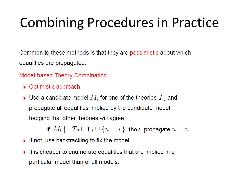
59. Combining Procedures in Practice

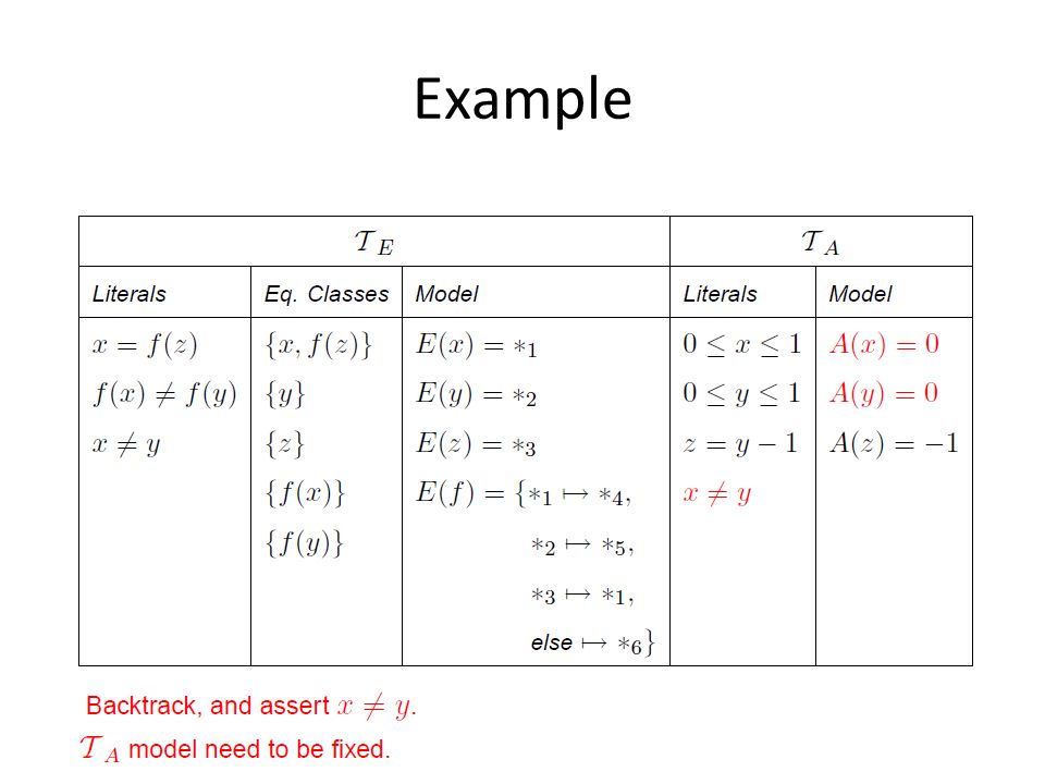
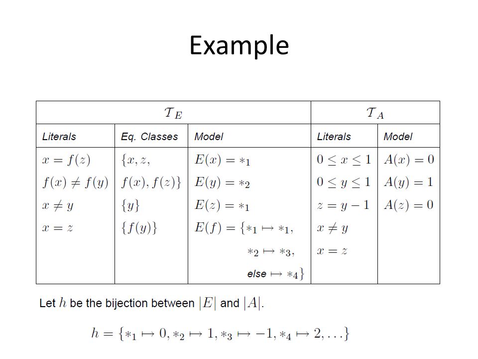
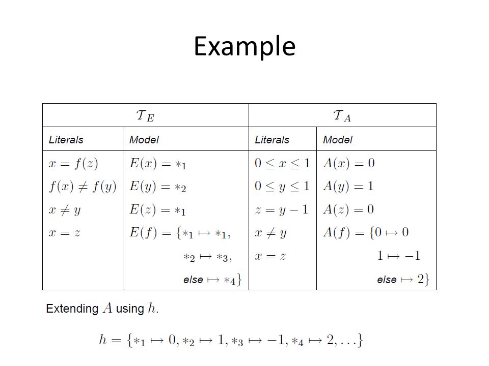
61. Example

70. Summary Main SMT solvers apply CDCL style refinement search of models & proofs. Efficient SMT solvers rely on propagation and filters to control theory reasoning (instantiating theory axioms). Combining solvers rely on compositional glue (e.g., by sharing equalities).

71. HORN CLAUSES AND STATE MACHINES

72. mc(x) = x-10 if x > 100 mc(x) = mc(mc(x+11)) if x  100 assert (x ≤ 101  mc(x) = 91) Symbolic model checking as Satisfiability of Horn Clauses

73. Program Verification (Safety) as Solving fixed-points asSatisfiability of Horn clauses Program Verification as SMT [Bjørner, McMillan, Rybalchenko, SMT workshop 2012] Hilbert Sausage Factory: [Grebenshchikov, Lopes, Popeea, Rybalchenko, PLDI 2012]