1. 15_01fig_PChem.jpg Particle in a Box

2. Recall 15_01fig_PChem.jpg Particle in a Box

3. 15_01fig_PChem.jpg Particle in a Box Initial conditions Recall

4. 15_02fig_PChem.jpg Wavefunctions for the Particle in a Box Normalization Recall Therefore a

5. Recall 15_02fig_PChem.jpg Wavefunctions are Orthonormal + - + Even Odd + - + Even Odd + - + -

6. 15_02fig_PChem.jpg Wavefunctions are Orthonormal AND

7. 15_03fig_PChem.jpg Orthogonal Normalized + - Node # nodes = n-1 n > 0 Wavelength + + + + Ground state Particle in a Box Wavefunctions n=1 n=2 n=3 n=4

8. 15_02fig_PChem.jpg Probabilities Independent of n For 0 <x < a/2 Recall

9. 15_02fig_PChem.jpg Expectation Values Average position Independent of n Recall as 2ca=2  n From a table of integrals

10. 15_02fig_PChem.jpg Expectation Values From a table of integrals or from Maple.

11. 15_02fig_PChem.jpg Expectation Values oddeven

12. 15_02fig_PChem.jpg Expectation Values Recall

13. Uncertainty Principle

14. Free Particle k is determined by the initial velocity of the particle, which can be any value as there are no constraints imposed on it. Therefore k is a continuous variable, which implies that E,  and  are also continuous. This is exactly the same as the classical free particle. Two travelling waves moving in the opposite direction with velocity v.

15. Probability Distribution of a Free Particle Wavefunctions cannot be normalized over Let’s consider the interval The particle is equally likely to be found anywhere in the interval

16. 15_04fig_PChem.jpg Classical Limit Probability distribution becomes continuous in the limit of infinite n, and also with limited resolution of observation.

17. 15_p19_PChem.jpg Particle in a Two Dimensional Box x y 0,0 a,0 0,b a,b Product wavefunction

18. 15_p19_PChem.jpg Particle in a Two Dimensional Box Separable

19. Particle in a Two Dimensional Box

20. Particle in a Square Box 1 1 2 3 1 3 2 2 5 1 1 2 03 2 2 41 213 108 265 Quantum Numbers Number of Nodes Energy

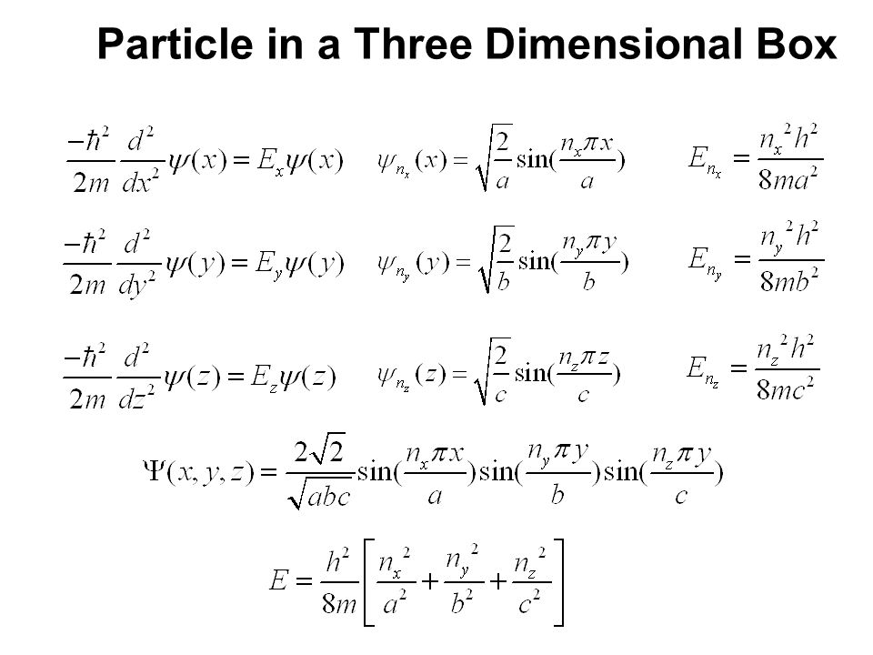
21. Particle in a Three Dimensional Box

23. Free Electron Models R R L 6  electrons HOMO LUMO EE

24. 16_01tbl_PChem.jpg Free Electron Models n H = 2 345 nm 375 nm 390 nm max n H = 3 n H = 4

25. Particle in a Finite Well Inside the box

26. Particle in a Finite Well Classically forbidden region as KE E n Limited number of bound states. WF penetrates deeper into barrier with increasing n. A,B, A’ B’ & C are determined by V o, m, a, and by the boundary and normalization conditions. Note: not ikx !!!

27. 16_03fig_PChem.jpg Core and Valence Electrons Weakly bound states - Wavefunctions extend beyond boundary. - Delocalized (valence)- Have high energy. - Overlap with neighboring states of similar energy Strongly bound states – Wavefunctioons are confined within the boundary - Localized. (core)- Have lower energy Two Free Sodium Atoms In the lattice x e -lattice spacing

28. 16_05fig_PChem.jpg Conduction Bound States (localized) Unbound states Occupied Valence States- Band Unoccupied Valence States - Band electrons flow to + increased occupation of val. states on + side Consider a sodium crystal sides 1 cm long. Each side is 2x10 7 atoms long. Sodium atoms Energy spacing is very small w.r.t, thermal energy, kT. Energy levels form a continuum Valence States (delocalized) bias

29. 16_08fig_PChem.jpg Tunneling Decay Length = 1/  The higher energy states have longer decay lengths The longer the decay length the more likely tunneling occurs The thinner the barrier the more likely tunneling occurs

30. 16_09fig_PChem.jpg Scanning Tunneling Microscopy Tip Surface work functions no contact Contact Contact with Applied Bias Tunneling occurs from tip to surface

31. 16_11fig_PChem.jpg Scanning Tunneling Microscopy

32. 16_13fig_PChem.jpg Tunneling in Chemical Reactions The electrons tunnel to form the new bond Small tunnelling distance relatively large barrier

33. 16_14fig_PChem.jpg Quantum Wells States Allowed Fully occupied No States allowed States are allowed Empty in Neutral X’tal. Alternating layers of Al doped GaAs with GaAs 3D Box a = 1 to 10 nm thick b = 1000’s nm long & wide Energy levels for y and z - Continuous Energy levels for x - Descrete 1D Box along x !! Band Gap of Al doped GaAs > Band Gap GaAs Cond. Band GaAs < Cond. Band Al Doped GaAs e’s in Cond. Band of GaAS in energy well. Semi Conductor

34. 16_14fig_PChem.jpg Quantum Wells finite barrier QW Devices can be manufactured to have specific frequencies for application in Lasers.  E ex < Band Gap energy Al doped GaAS  E ex > Band Gap energy GaAS EE

35. 16_16fig_PChem.jpg Quantum Dots Crystalline spherical particles1 to 10 nm in diameter. Band gap energy depends on diameter Easier and cheaper to manufacture 3D PIB !!!

36. 16_18fig_PChem.jpg Quantum Dots

37. Quantum Dot Solar Cells Dye Sensitized Solar Cell

38. Background Organic Polymer Solar Cells Fullerenes(Acceptor) Organic polymer (Donor) Organic polymersFullerene(PCBM)