1. -Imagine a typical ‘mixer’ party, where one of the guests knows a bit of gossip that everyone would like to know. -Assuming that people tell this gossip to the people they meet at the party: a)How many people would eventually hear the gossip? b)How long would it take to spread through the group? The Cocktail Party Problem Relational Dynamics of Diffusion

2. The Cocktail Party Problem -Some specifics to narrow down the problem. - 30 people invited, party lasts an hour. -At any given moment in time, you can only carry on a conversation with 3 other people -Guests mingle well – they spend a short time talking to most people, but a long time to a small number (such as their date). -Mingling is somewhat space-based – you talk to the people you bump into, then move on to someone else after a short time. -The bit of gossip moves instantaneously across connected sets (so time-to-diffuse=0). Relational Dynamics of Diffusion

3. -Some specifics to narrow down the problem. A (seemingly) simple network problem: record who talks to who, and map the network. Mean distance: 1.99 Diameter: 4 steps The Cocktail Party Problem Relational Dynamics of Diffusion

4. -But such an image conflates many temporally distinct events. A more accurate image is something like this: In general, the graphs over which diffusion happens often: Have timed edges Nodes enter and leave Edges can re-occur multiple times Edges can be concurrent These features break transmission paths, generally lowering diffusion potential – and opening a host of interesting questions about the intersection of structure and time in networks. The Cocktail Party Problem Relational Dynamics of Diffusion

5. When is a network? Source: Bender-deMoll & McFarland “The Art and Science of Dynamic Network Visualization ” JoSS 2006

6. When is a network? At the finest levels of aggregation networks disappear, but at the higher levels of aggregation we mistake momentary events as long-lasting structure. Is there a principled way to analyze (and visualize) networks where the edges are dynamic? There is unlikely to be a single answer for all questions, but the set of types of questions might be manageable: Structural change (networks as dynamic objects of study). The interest is in mapping changes in the topography of the network, to see model how the field itself changes over time. Ultimately, this has to be linked to questions about how network macro- structures emerge as the result of actor behavior rules. Diffusion and flow (networks as resources or constraints for actors): The timing of relations affects flow in a way that changes many of our standard measures. If our interest is in “Relational ties [as] channels for transfer or flow of resources” (W&F p.4), then we can use the diffusion process to shape our analyses.

7. Time and Social Networks Historically, time has been incorporated into the network by looking at (a) changes in the distribution of an item over the population, over time (I.e. the adoption of an innovation, the spread of an idea, etc.) (b) different cross-sectional slices of the network (I.e. world system in 1965, 1975, 1985 or protest networks over time). These approaches take us a long way. They don’t allow us to explicitly model the changes within the network, or explain changes in the distribution of goods as a function of relationship timing. This static bias is built into some views of the network (think of Wellman’s definition as patterns of stable relations). What we want is to be able to account for the dynamics of the network in “real time” -- to account for changes in relations as a function of changes in relations occurring around ego.

8. Time and Social Networks Examples of looking at change in networks: Roy and interlocking directorates (ASR 1983, 248-257) Non-financial interlocks: 1886 - 1890

9. Time and Social Networks Examples of looking at change in networks: Roy and interlocking directorates (ASR 1983, 248-257) Non-financial interlocks: 1891 - 1895

10. Time and Social Networks Examples of looking at change in networks: Roy and interlocking directorates (ASR 1983, 248-257) Non-financial interlocks: 1896 - 1900

11. Time and Social Networks Examples of looking at change in networks: Roy and interlocking directorates (ASR 1983, 248-257) Non-financial interlocks: 1901 - 1905

12. Bearman and Everett: The Structure of Social Protest 1 3 2 4 5 6 1 3 2 4 5 7 6 1 3 2 4 5 (‘61-63) (‘66-68) (‘71-73) 7 6 1 3 2 4 5 (‘76-78) (‘81-83) 7 5 1 6 3 4 2 See paper for group compositions

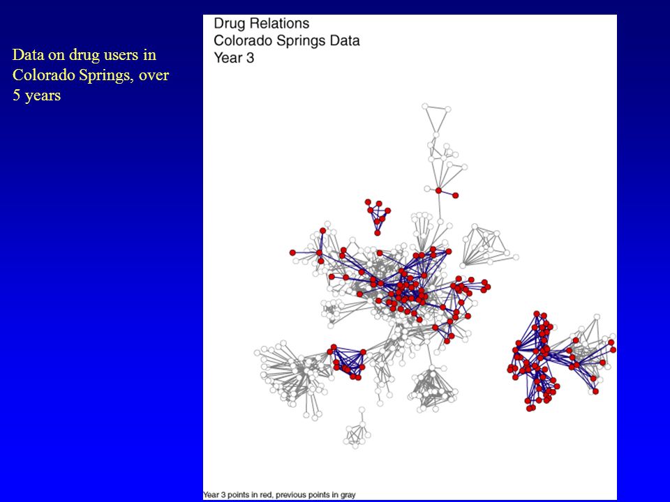
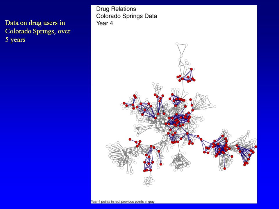
13. Data on drug users in Colorado Springs, over 5 years

18. An alternative approach to visualizing time in networks involves dynamic network displays. Moody, McFarland and Bender-deMoll have worked on this, linked to the SoNIA software. Theoretically, we are interested in being able to see the holistic changes in networks that might be missed with any display of summary statistics. This involves the development of a new dynamic language for networks, moving from words describing stable ‘structures’ to words that describe change: Pace Tempo Rhythm Etc.

19. Freeman’s animation of change based on an early ‘email’ system in the 1970s. (note: the animation runs twice: once without groups, once by groups)

20. Animation as a tool: SoNIA Challenge:

21. Animation as a tool: SoNIA Solution:

22. Animation as a tool: SoNIA Challenge:

23. Animation as a tool: SoNIA Solution:

24. Animation as a tool: SoNIA Challenge:

25. Animation as a tool: SoNIA Solution:

26. Animation as a tool: SoNIA Challenge:

27. Animation as a tool: SoNIA Solution:

28. http://csde.washington.edu/statnet/movies/ConcurrencyAndReachability.mov Animation captures much of the dynamism we care about: STD Diffusion Representing dynamic networks?

29. Animation captures much of the dynamism we care about: Representing dynamic networks?

30. Animation captures much of the dynamism we care about: Representing dynamic networks?

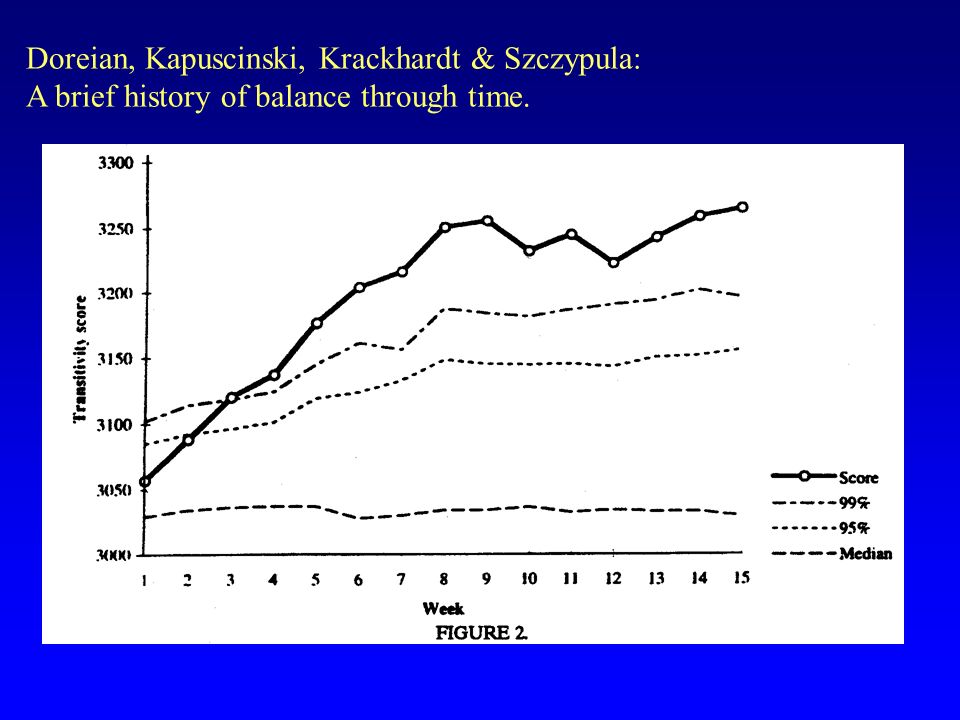
31. Doreian, Kapuscinski, Krackhardt & Szczypula: A breif history of balance through time. Reanalyzes the Newcomb fraternity data, to look at changes in social balance over time. The basic balance theory hypothesis is that people who find themselves in an unbalanced position should change their relations to generate balance. Hypothetically, this should lead to greater balance over time. After discussing a set of problems imposed because the data are forced ranks, they first look at simple reciprocity.

32. Doreian, Kapuscinski, Krackhardt & Szczypula: A brief history of balance through time.

34. 40 30 20 10 0 123456789 11121314 Week % Change in ties Relational Stability

35. Moody, McFarland & BenderdeMoll re-analyze the same data:

37. An extension: A balance model of friendship change among adolescents The basic hypothesis of social balance is that people will make choices that bring the entire group into balance. But, consider how a given relationship looks from different perspectives: A transition that generates transitivity for one person can generate intransitivity for another. As such, there is no guarantee that friendship change will result in a globally balanced outcome.

38. Here, we see that it is possible, even within the triad, for a transition to be transitive, but the state to be negative, which implies that one person’s transitive change is another’s intransitive.

39. Animation captures much of the dynamism we care about: Seeking Social Balance Source: Moody, James, Daniel A. McFarland and Skye Bender-DeMoll (2005) "Dynamic Network Visualization: Methods for Meaning with Longitudinal Network Movies” American Journal of Sociology 110:1206-1241 Representing dynamic networks?

40. The Balance Model works for objects too: Source: Moody, James, Daniel A. McFarland and Skye Bender-DeMoll (2005) "Dynamic Network Visualization: Methods for Meaning with Longitudinal Network Movies” American Journal of Sociology 110:1206-1241 Representing dynamic networks? Achieved Characteristics – ties from circles to squares can change

41. The Balance Model works for objects too: Source: Moody, James, Daniel A. McFarland and Skye Bender-DeMoll (2005) "Dynamic Network Visualization: Methods for Meaning with Longitudinal Network Movies” American Journal of Sociology 110:1206-1241 Representing dynamic networks? Ascribed Characteristics – ties from circles to squares cannot change

42. The Balance Model works for objects too: Source: Moody, James, Daniel A. McFarland and Skye Bender-DeMoll (2005) "Dynamic Network Visualization: Methods for Meaning with Longitudinal Network Movies” American Journal of Sociology 110:1206-1241 Representing dynamic networks? Democrat Smoke What happens next?

43. Willard Van Quine, professor of philosophy and mathematics emeritus from Harvard University who is regarded as one of the four most famous living philosophers in the world, wrote his doctoral thesis on a 1927 Remington typewriter, which he still uses. However, he "had an operation on it" to change a few keys to accommodate special symbols. "I found I could do without the second period, the second comma -- and the question mark.” "You don't miss the question mark?” "Well, you see, I deal in certainties." Selection or Influence?

44. Selection That some unobserved factor, z, creates both friendships and the outcome of interest. Endogeneity That the causal order of peer relations and outcomes is reversed. Peers do not cause Y, but Y causes friendship relations Selection or Influence?

45. Selection What do we know about how friendships form? Opportunity / focal factors - Being members of the same group - In the same class - On the same team - Members of the same church Structural Relationship factors - Reciprocity - Social Balance Behavior Homophily - Smoking - Drinking

46. Selection How to correct this problem? Essentially, this is an omitted variable problem, and my “solution” has been to identify as many potentially relevant alternative variables as I can find.

47. Endogeneity Estimated: Y =  0 +  1 (P) +  where P = some peer function. But the actual model may really be: P =  ’ 0 +  ’ 1 (Y) + 

48. Algebraically the relation between y and p should be direct translation of the coefficients since: Endogeneity Does it matter? The statistical problem of endogeneity is that when you estimate  ’ 1, it does not equal 1/  1, because of our assumptions about x, and hence . (see Joel H. Levine, Exceptions are the Rule, for a full discussion of this)

49. Endogeneity Fully specified peer influence models: Where W is a matrix of interpersonal weights, calculated from the friendship adjacency matrix (the mixed-regressive autoregressive peer influence model, see Friedkin 1999, chapter 2, Doreian, 1982, SMR) These models can be estimated directly with Add Health data, but again the problem is that W may be determined by Y.

50. Endogeneity Possible solutions: Theory: Given what we know about how friendships form, is it reasonable to assume a bi- directional cause? That is, work through the meeting, socializing, etc. process and ask whether it makes sense that Y is a cause of W. Models: - Time Order. We are on somewhat firmer ground if W precedes Y in time. Thus, using the in-school friendship structure to predict wave 1 outcomes is useful. - Simultaneous Models. Model both the friendship pattern and the outcome of interest simultaneously.

51. Endogeneity Simultaneous models: Temporal Lag models: ERGM’s with edge/dyad covariates for prior exposure & contact. Simple & direct way to express change as a model & look for consistency One way to do this is with SEMs, but for identification, you must find some variables that predict friendship that do not also predict Y, which given the very nature of the endogeneity problem, is hard to do. Could also model a mixed “network” of relations and behaviors using dyads and an ERGM-style model to predict “ties” within the joint network

52. Endogeneity Simple time-lag model: Prosper Peers

53. Endogeneity Simple time-lag model

54. Endogeneity A mixed selection and influence model: Simultaneous balance on friendship and behavior. Two linked models: a) actors seek interpersonal balance among friends b) actors change their opinions / behaviors as a weighted function of the people they are tied to, with W weighted by number of transitive ties Positive to attribute Negative to attribute Friendship Attribute Actor

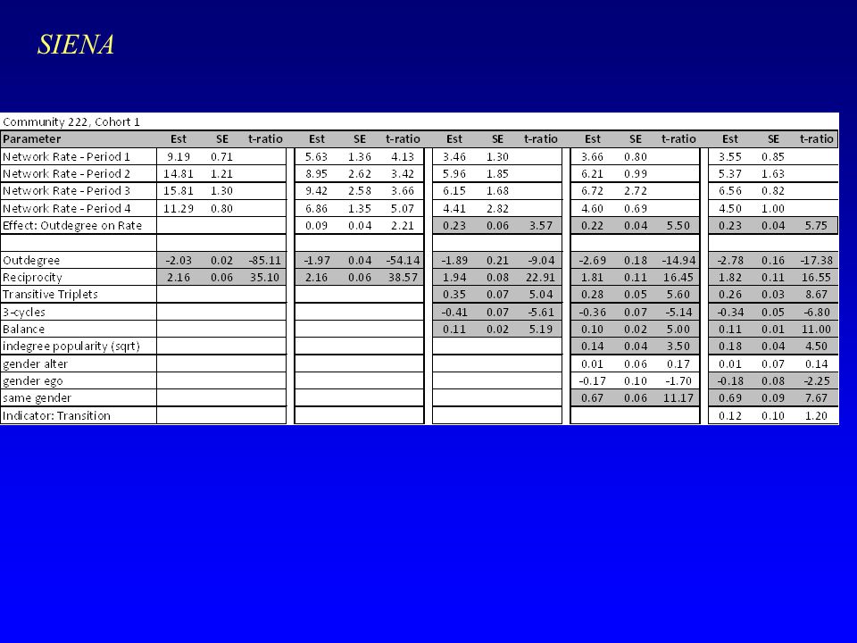
55. SIENA

57. When is a network? At the finest levels of aggregation networks disappear, but at the higher levels of aggregation we mistake momentary events as long-lasting structure. Is there a principled way to analyze (and visualize) networks where the edges are dynamic? There is unlikely to be a single answer for all questions, but the set of types of questions might be manageable: Structural change (networks as dynamic objects of study). The interest is in mapping changes in the topography of the network, to see model how the field itself changes over time. Ultimately, this has to be linked to questions about how network macro- structures emerge as the result of actor behavior rules. Diffusion and flow (networks as resources or constraints for actors): The timing of relations affects flow in a way that changes many of our standard measures. If our interest is in “Relational ties [as] channels for transfer or flow of resources” (W&F p.4), then we can use the diffusion process to shape our analyses.

58. Diffusion through networks, when the network can change. A long tradition in network research focuses on social diffusion: how ideas, information or goods travel through a network. In almost all cases, the diffusion models rest on a network that is assumed to be constant. What are the implications for diffusion when the network structure can change? It turns out, that the timing of relations can have a huge impact on the possibility that things flow through the network. Best introduction to diffusion models: Coleman’s Introduction to Mathematical Sociology text Tom Valente’s Network Models of the Diffusion of Innovation

59. B C E DF A 2 - 5 3 - 7 0 - 1 8 - 9 3 - 5 A hypothetical Sexual Contact Network

60. B C E DF A The path graph for a hypothetical contact network

61. Direct Contact Network of 8 people in a ring

62. Implied Contact Network of 8 people in a ring All relations Concurrent Edge timing constraints on diffusion Reachability = 1.0 When is a network?

63. Implied Contact Network of 8 people in a ring Serial Monogamy (1) 1 2 3 7 6 5 8 4 Reachability = 0.71 Edge timing constraints on diffusion When is a network?

64. Implied Contact Network of 8 people in a ring Mixed Concurrent 2 2 1 1 2 2 3 3 Reachability = 0.57 Edge timing constraints on diffusion When is a network?

65. Implied Contact Network of 8 people in a ring Serial Monogamy (3) 1 2 1 1 2 1 2 2 Reachability = 0.43 Edge timing constraints on diffusion When is a network?

66. 1 2 1 1 2 1 2 2 Timing alone can change mean reachability from 1.0 when all ties are concurrent to 0.42. In general, ignoring time order is equivalent to assuming all relations occur simultaneously – assumes perfect concurrency across all relations. Edge timing constraints on diffusion When is a network?

67. Identifying the Minimum Path Density of a Graph It turns out that the safest network is one where relations are ‘inter-woven’ in a “early-late-earlier” pattern. To identify the paths empirically, you must search all possible paths in the network. t1t1 t1t1 t2t2 t2t2 t1t1 t1t1 t2t2 t2t2

68. An Empirical Example

70. Relationship timing constrains diffusion paths because goods can only move forward in time. ab c d Standard graph: - Connected component - Everyone could diffuse to everyone else When is a network?

71. Relationship timing constrains diffusion paths because goods can only move forward in time. ab Dynamic graph: - Edges start and end - Can’t pass along an edge that has ended Time b c c d When is a network?

72. Relationship timing constrains diffusion paths because goods can only move forward in time. ab Dynamic graph: - Edges start and end - Can’t pass along an edge that has ended Diffusion is asymmetric: a can reach c (through b) and b and reach d (through c), but not the other way around. Time b c c d When is a network?

73. Relationship timing constrains diffusion paths because goods can only move forward in time. Time abc c d Concurrency, when edges share a node at the same time, allows diffusion to move symmetrically through the network. This can have a dramatic effect on increasing the down-stream potential for any give tie. When is a network?

74. A B C D E F A 0 1 2 2 4 1 B 1 0 1 2 3 2 C 0 1 0 1 2 2 D 0 0 1 0 1 1 E 0 0 0 1 0 2 F 1 0 0 1 0 0 While a is 2 steps from d, and d is 1 step from e, a and e are 4 steps apart. This is because a shorter path from a to e emerges after the path from d to e ended. 4 2 1 Path distances no longer simply add When is a network? Changing Paths

75. Timing constrains potential diffusion paths in networks, since bits can flow through edges that have ended. This means that: Structural paths are not equivalent to the diffusion-relevant path set. Network distances don’t build on each other. Weakly connected components overlap without diffusion reaching across sets. Small changes in edge timing can have dramatic effects on overall diffusion Diffusion potential is maximized when edges are concurrent and minimized when they are “inter-woven” to limit reachability. Combined, this means that many of our standard path-based network measures will be incorrect on dynamic graphs. When is a network? Changing Paths

76. The distribution of paths is important for many of the measures we typically construct on networks, and these will be change if timing is taken into consideration: Centrality: Closeness centrality Path Centrality Information Centrality Betweenness centrality Network Topography Clustering Path Distance Groups & Roles: Correspondence between degree-based position and reach-based position Structural Cohesion & Embeddedness Opportunities for Time-based block-models (similar reachability profiles) In general, any measures that take the systems nature of the graph into account will differ. When is a network? Changing Paths

77. New versions of classic reachability measures: 1)Temporal reach: The ij cell = 1 if i can reach j through time. 2)Temporal geodesic: The ij cell equals the number of steps in the shortest path linking i to j over time. 3)Temporal paths: The ij cell equals the number of time-ordered paths linking i to j. These will only equal the standard versions when all ties are concurrent. When is a network? Diffusion: What do networks do?

78. Duration explicit measures 4)Quickest path: The ij cell equals the shortest time within which i could reach j. 5)Earliest path: The ij cell equals the real-clock time when i could first reach j. 6)Latest path: The ij cell equals the real-clock time when i could last reach j. 7) Exposure duration: The ij cell equals the longest (shortest) interval of time over which i could transfer a good to j. Each of these also imply different types of “betweenness” roles for nodes or edges, such as a “limiting time” edge, which would be the edge whose comparatively short duration places the greatest limits on other paths. When is a network? Diffusion: What do networks do?

79. Define time-dependent closeness as the inverse of the sum of the distances needed for an actor to reach others in the network. * Actors with high time-dependent closeness centrality are those that can reach others in few steps given temporal order. Note this is directed. Since D ij =/= D ji (in most cases) once you take time into account. * If i cannot reach j, I set the distance to n+1 When is a network? Diffusion: What do networks do?

80. Define fastness centrality as the average of the clock-time needed for an actor to reach others in the network: Actors with high fastness centrality are those that would reach the most people early. These are likely important for any “first mover” problem. When is a network? Diffusion: What do networks do?

81. Define quickness centrality as the average of the minimum amount of time needed for an actor to reach others in the network: Where T jit is the time that j receives the good sent by i at time t, and T it is the time that i sent the good. This then represents the shortest duration between transmission and receipt between i and j. Note that this is a time-dependent feature, depending on when i “transmits” the good out into the population. The min is one of many functions, since the time-to-target speed is really a profile over the duration of t. When is a network? Diffusion: What do networks do?

82. Define exposure centrality as the average of the amount of time that actor j is at risk to a good introduced by actor i. Where T ijl is the last time that j could receive the good from i and T iif is the first time that j could receive the good from i, so the difference is the interval in time when i is at risk from j. When is a network? Diffusion: What do networks do?

83. How do these centrality scores compare? Here I compare the duration-dependent measures to the standard measures on this example graph. Based only on the structure of the ties, this graph has lots of different centers, depending on closeness, betweenness or degree. In this graph, closeness and betweenness correlate at 0.64, closeness and degree at 0.56, and betweeness and degree at 0.71 Node size proportional to degree When is a network? Diffusion: What do networks do?

84. Network Dynamics & Flow How do these centrality scores compare? Here I compare the duration-dependent measures to the standard measures on this example graph. But these edges are timed, since publications occur at a particular date. Here I treat the edges as lasting between the first and last publication date, and animate the resulting network. Dark blue edges are active, past edges are “ghosted” onto the map. Make note of the fairly high concurrency (some of it necessary due to two-mode data).

85. Simulate time structure on a small sample of real graphs. These graphs are small walks (~100 nodes) from the soc coauthor network. Construct times and durations as: Assign starting times to edges as a random draw from a uniform distribution. Mean concurrency levels are set by compressing or stretching the starting-time distribution. Each edge is given a duration drawn from a skewed distribution Record the node-level dynamic position measures Here I focus on Time-closeness centrality Correlate the time-sensitive score to the fixed score. Does timing matter? How wrong are we if we ignore it? When is a network?

86. Network Dynamics & Flow How do these centrality scores compare? What is the relation between structural centrality and duration centrality? Here for the observed edge timings.

87. Network Dynamics & Flow How do these centrality scores compare? Box plots based on 500 permutations of the observed time durations, which holds constant the duration distribution and the number of edges active at any given time. Correlation w. Closeness centrality 0.2 0.4 0.6

88. Network Dynamics & Flow How do these centrality scores compare? The “most important actors” in the graph depend crucially on when they are active. The correlations can range wildly over the exact same contact structure. Concurrency is important, but not determinant (at least within the range studied here). We need to extend our intuition on the global distribution of time in the graph.

89. How does the low correlation between structural and temporal measures vary by the contact structure? Are some sorts of structures more “robust to time” than others? Test this by: 1) Examine the variability in diffusion potential across structures. Diffusion potential is measured by the proportion of pairs reachable in the network: 1 2 1 1 2 1 2 2 Reachability = 0.43 When is a network? Robust Diffusion: When does timing matter most/least? 2) What types of positions within networks have low time-related variance?

90. Proportion of pairs reachable through times Min reachability Low Medium High Concurrency When is a network? Robust Diffusion: When does timing matter most/least?

91. Relative Reach – Reachability over minimum possible When is a network? Robust Diffusion: When does timing matter most/least?

92. Relative Reach – Reachability over minimum possible Low Medium High Concurrency When is a network? Robust Diffusion: When does timing matter most/least?

93. Volume Distance Connectivity Nodes: 83 Mean Deg: 3.04 Density: 0.037 Centralization: 0.237 Nodes: 148 Mean Deg: 6.16 Density: 0.042 Centralization: 0.187 Nodes: 80 Mean Deg: 5.27 Density: 0.067 Centralization: 0.373 Nodes: 154 Mean Deg: 3.71 Density: 0.025 Centralization: 0.147 Nodes: 128 Mean Deg: 3.39 Density: 0.027 Centralization: 0.205 Mean: 0.398 Diameter: 6 Centralization: 0.321 Mean: 3.59 Diameter: 5 Centralization: 0.312 Mean: 3.02 Diameter: 5 Centralization: 0.413 Mean: 4.99 Diameter: 8 Centralization: 0.259 Mean: 4.55 Diameter: 6 Centralization: 0.301 Largest BC:0.16 Pairwise K: 1.07 Largest BC: 0.51 Pairwise K: 1.57 Largest BC: 0.33 Pairwise K: 1.34 Largest BC: 0.08 Pairwise K: 1.07 Largest BC: Pairwise K: 1.06 When is a network? Robust Diffusion: When does timing matter most/least?

94. K=1 K=2 K=3 K=4 K=1 N=10 K=2 N=9 K=3 N=4 K=4 N=5 1 2 3 4 5 6 7 8 9 0 1. 3 3 3 2 2 2 2 2 1 2 3. 3 3 2 2 2 2 2 1 3 3 3. 3 2 2 2 2 2 1 4 3 3 3. 2 2 2 2 2 1 5 2 2 2 2. 4 4 4 4 1 6 2 2 2 2 4. 4 4 4 1 7 2 2 2 2 4 4. 4 4 1 8 2 2 2 2 4 4 4. 4 1 9 2 2 2 2 4 4 4 4. 1 10 1 1 1 1 1 1 1 1 1. Average K = 2.38 When is a network? Robust Diffusion: When does timing matter most/least?

95. 4 clustered networks w. different global connectivity Net1 Net2 Net3 Net4 Kcon: 2.95 Kcon: 1.55 Kcon: 2.43Kcon: 1.36 When is a network?

96. Relative (to min) Reachability When is a network? Robust Diffusion: When does timing matter most/least?

97. 1 2 3 4 5 6 7 11.522.53 Pairwise k Connectivity Mean Relative Reach Interaction of Structure and Time When is a network? Robust Diffusion: When does timing matter most/least?

98. Small World Mechanisms on Dynamic Graphs

99. Concurrency opens paths for diffusion to move reciprocally. Small World Mechanisms on Dynamic Graphs Use concurrency to adjust the temporal structure of the graph.

100. Small World Mechanisms on Dynamic Graphs Simulation setup: 1.Generate a 200 node ring lattice, where every node has 6 ties. 2.Assign starting times to edges as a random draw from a uniform distribution. Mean concurrency levels are set by compressing or stretching the starting-time distribution. 3.Each edge is given a duration drawn from a skewed distribution. 4.Once edge-times are set, randomly rewire the graph by reassigning one end of the edge to a node chosen at random. 5.Calculate the reachability and mean distance scores for each rewiring. 6.Repeat 4-5 many times, increasing the number of edges rewired. Simulation varies the proportion of edges rewired and the level of graph concurrency in the network.

101. Small World Mechanisms on Dynamic Graphs

102. The rapid shortening of distance we typically see in small-world simulations does not occur in dynamic networks. The initial distances are much higher, since many nodes are not reachable. The rapid decreasing marginal returns to rewiring are much slower When concurrency is relatively low, the effects of rewiring are nearly linear When concurrency is relatively high, the characteristic curve starts to emerge, but is much less steep. Note all of these concurrency levels are non-trivial. Even when only 4% of two-paths in the graph are concurrent, nearly 50% of nodes have at least 1 concurrent edge. Why?

103. Small World Mechanisms on Dynamic Graphs Why do we see this pattern? Long distant out-reach is rare: Consider a set of typical reach-paths in a dynamic network with time- disjoint edges: e1e1 p 1  2 = p(e 2 > e 1 ) e2e2 p 2  3 = p(e 3 > e 2 ) e3 p 3  4 = p(e 4 > e 3 ) e1e1 e2e2 e3e3 e4e4 P 3  4 < p 2  3 < p 1  2 < 1.0 Time 

104. Small World Mechanisms on Dynamic Graphs Why do we see this pattern? Long distant out-reach is rare: If we allow concurrency & lengthen the duration of edges (proportionate to the observation window): e1e1 p 1  2 = p(e 2 > e 1 ) e2e2 p 2  3 = p(e 3 > e 2 ) e3 p 3  4 = p(e 4 > e 3 ) e1e1 e2e2 e3e3 e4e4 P i  j is still decreasing, but not as rapidly. Time 

105. Small World Mechanisms on Dynamic Graphs Why do we see this pattern? Long distant out-reach is rare: If we allow concurrency & lengthen the duration of edges (proportionate to the observation window): e1e1 p 1  2 = p(e 2 > e 1 ) e2e2 p 2  3 = p(e 3 > e 2 ) e3 p 3  4 = p(e 4 > e 3 ) e1e1 e2e2 e3e3 e4e4 P i  j is constant Time 

106. How do we capture the fully dynamic nature of networks? Source: Bender-deMoll & McFarland “The Art and Science of Dynamic Network Visualization ” JoSS 2006

107. Temporal projections of “net-time” Time-Space graph representations “Stack” a dynamic network in time, compiling all “node-time” and “edge- time” events (similar to an event-history compilation of individual level data). Consider an example: Representing dynamic networks? a)Repeat contemporary ties at each time observation, linked by relational edges as they happen. b)Between time slices, link nodes to later selves “identity” edges

108. a)Repeat contemporary ties at each time observation, linked by relational edges as they happen. b)Between time slices, link nodes to later selves “identity” edges Time-Space graph representations “Stack” a dynamic network in time, compiling all “node-time” and “edge- time” events (similar to an event-history compilation of individual level data). Consider an example: Example from Skye Bender-deMoll Temporal projections of “net-time” Representing dynamic networks?

109. Time-Space graph representations “Stack” a dynamic network in time, compiling all “node-time” and “edge- time” events (similar to an event-history compilation of individual level data). Consider an example: Representing dynamic networks? a)Repeat contemporary ties at each time observation, linked by relational edges as they happen. b)Between time slices, link nodes to later selves “identity” edges

110. a)Rotating a T-S graph to look “into” time (z axis) lets you compare relative space trajectories, as nodes move past each other in the space. A sort of “animation trace” Time-Space graph representations “Stack” a dynamic network in time, compiling all “node-time” and “edge- time” events (similar to an event-history compilation of individual level data). Consider an example: Representing dynamic networks?

111. Fully-sequenced data with fine time-stamps: Condense the graph by using identity edges to link to nodes whenever they change a relation, so you capture just the start and end of each instance of a relation. - Concurrency pops out as strong components > 2 nodes. - Relation duration as length of identity edges -tempo as marginal distribution of start/end over time. Time-Space graph representations “Stack” a dynamic network in time, compiling all “node-time” and “edge- time” events (similar to an event-history compilation of individual level data). Collapsed time-labeled view becomes… Representing dynamic networks?

112. Fully-sequenced data with fine time-stamps: Condense the graph by using identity edges to link to nodes whenever they change a relation, so you capture just the start and end of each instance of a relation. - Concurrency pops out as strong components > 2 nodes. - Relation duration as length of identity edges -tempo as marginal distribution of start/end over time. Time-Space graph representations “Stack” a dynamic network in time, compiling all “node-time” and “edge- time” events (similar to an event-history compilation of individual level data). …a TSG graph (arranged in social space) … Representing dynamic networks?

113. Fully-sequenced data with fine time-stamps: Condense the graph by using identity edges to link to nodes whenever they change a relation, so you capture just the start and end of each instance of a relation. - Concurrency pops out as strong components > 2 nodes. - Relation duration as length of identity edges -tempo as marginal distribution of start/end over time. Time-Space graph representations “Stack” a dynamic network in time, compiling all “node-time” and “edge- time” events (similar to an event-history compilation of individual level data). …arranged in time. Representing dynamic networks?

114. Example School Sequence Pooled “time- space” network with students at each wave linked to themselves later in time. Nodes colored by first school at which they appear in the sample. Isolates not represented here… Positional Models: Explorations of Dynamic Settings

115. Consider a comparison: Baboon Politics Representing dynamic networks?

116. So now we: 1)Convert every edge to a node 2)Draw a directed arc between edges that (a) share a node and (b) precede each other in time. This is still cumbersome, so we can further condense by shifting our attention from nodes to edges, creating a timed line graph Consider an example: Representing dynamic networks?

117. So now we: 1)Convert every edge to a node 2)Draw a directed arc between edges that (a) share a node and (b) precede each other in time. 3)After the transformation, concurrent relations are easily seen as reciprocal edges in the line-graph. So this….. This is still cumbersome, so we can further condense by shifting our attention from nodes to edges, creating a timed line graph Representing dynamic networks?

118. So now we: 1)Convert every edge to a node 2)Draw a directed arc between edges that (a) share a node and (b) precede each other in time. 3)After the transformation, concurrent relations are easily seen as reciprocal edges in the line-graph. Becomes this: This is still cumbersome, so we can further condense by shifting our attention from nodes to edges, creating a timed line graph Representing dynamic networks?

119. Line-graph advantages: Technical: Reduces the size of the time-space expansion drastically Theoretical: Moves us to a purely relational space. “Actors” dissolve into paths along edges. And, since paths cross, we can literally operationalize “self” and “other” as dependant on intersection. Representing dynamic networks?

120. The Mingle Mixing Problem Space