Download presentation
Presentation is loading. Please wait.

1
2.4 Linear Independence (線性獨立) and Linear Dependence(線性相依)
A linear combination(線性組合) of the vectors in V is any vector of the form c1v1 + c2v2 + … + ckvk where c1, c2, …, ck are arbitrary scalars. A set of V of m-dimensional vectors is linearly independent(線性獨立) if the only linear combination of vectors in V that equals 0 is the trivial linear combination. A set of V of m-dimensional vectors is linearly dependent (線性相依) if there is a nontrivial linear combination of vectors in V that adds up to 0.
 of the vectors in V is any vector of the form c1v1 + c2v2 + … + ckvk where c1, c2, …, ck are arbitrary scalars. A set of V of m-dimensional vectors is linearly independent(線性獨立) if the only linear combination of vectors in V that equals 0 is the trivial linear combination. A set of V of m-dimensional vectors is linearly dependent (線性相依) if there is a nontrivial linear combination of vectors in V that adds up to 0.")
2
Example 10: LD Set of Vectors (p.33)
Show that V = {[ 1 , 2 ] , [ 2 , 4 ]} is a linearly dependent set of vectors. Solution Since 2([ 1 , 2 ]) – 1([ 2 , 4 ]) = (0 0), there is a nontrivial linear combination with c1 =2 and c2 = -1 that yields 0. Thus V is a linear dependent set of vectors.
 – 1([ 2 , 4 ]) = (0 0), there is a nontrivial linear combination with c1 =2 and c2 = -1 that yields 0. Thus V is a linear dependent set of vectors.")
3
Linear dependent 線性相依 (p.33)
What does it mean for a set of vectors to linearly dependent? A set of vectors is linearly dependent only if some vector in V can be written as a nontrivial linear combination of other vectors in V. If a set of vectors in V are linearly dependent, the vectors in V are, in some way, NOT all “different” vectors. By “different” we mean that the direction specified by any vector in V cannot be expressed by adding together multiples of other vectors in V. For example, in two dimensions, two linearly dependent vectors lie on the same line.

4
The Rank of a Matrix (p.34) Let A be any m x n matrix, and denote the rows of A by r1, r2, …, rm. Define R = {r1, r2, …, rm}. The rank(秩) of A is the number of vectors in the largest linearly independent subset of R. To find the rank of matrix A, apply the Gauss-Jordan method to matrix A. (Example 14, p.35) Let A’ be the final result. It can be shown that the rank of A’ = rank of A. The rank of A’ = the number of nonzero rows in A’. Therefore, the rank A = rank A’ = number of nonzero rows in A’.
 of A is the number of vectors in the largest linearly independent subset of R. To find the rank of matrix A, apply the Gauss-Jordan method to matrix A. (Example 14, p.35) Let A’ be the final result. It can be shown that the rank of A’ = rank of A. The rank of A’ = the number of nonzero rows in A’. Therefore, the rank A = rank A’ = number of nonzero rows in A’.")
5
Whether a Set of Vectors Is Linear Independent
A method of determining whether a set of vectors V = {v1, v2, …, vm} is linearly dependent is to form a matrix A whose ith row is vi. (p.35) - If the rank A = m, then V is a linearly independent set of vectors. - If the rank A < m, then V is a linearly dependent set of vectors.
 - If the rank A = m, then V is a linearly independent set of vectors. - If the rank A < m, then V is a linearly dependent set of vectors.")
6
2.5 The Inverse of a Matrix (反矩陣) (p.36)
A square matrix(方陣) is any matrix that has an equal number of rows and columns. The diagonal elements (對角元素)of a square matrix are those elements aij such that i=j. A square matrix for which all diagonal elements are equal to 1 and all non-diagonal elements are equal to 0 is called an identity matrix(單位矩陣). An identity matrix is written as Im.
 is any matrix that has an equal number of rows and columns. The diagonal elements (對角元素)of a square matrix are those elements aij such that i=j. A square matrix for which all diagonal elements are equal to 1 and all non-diagonal elements are equal to 0 is called an identity matrix(單位矩陣). An identity matrix is written as Im.")
7
The Inverse of a Matrix (continued)
For any given m x m matrix A, the m x m matrix B is the inverse of A if BA=AB=Im. Some square matrices do not have inverses. If there does exist an m x m matrix B that satisfies BA=AB=Im, then we write B= (p.39) The Gauss-Jordan Method for inverting an m x m Matrix A is Step 1 Write down the m x 2m matrix A|Im Step 2 Use EROs to transform A|Im into Im|B. This will be possible only if rank A=m. If rank A<m, then A has no inverse (p.40)
 The Gauss-Jordan Method for inverting an m x m Matrix A is. Step 1 Write down the m x 2m matrix A|Im. Step 2 Use EROs to transform A|Im into Im|B. This will be possible only if rank A=m. If rank A<m, then A has no inverse. (p.40)")
8
Matrix inverses can be used to solve linear systems. (example, p.40)
The Excel command =MINVERSE makes it easy to invert a matrix. Enter the matrix into cells B1:D3 and select the output range (B5:D7 was chosen) where you want A-1 computed. In the upper left-hand corner of the output range (cell B5), enter the formula = MINVERSE(B1:D3) Press Control-Shift-Enter and A-1 is computed in the output range
 where you want A-1 computed. In the upper left-hand corner of the output range (cell B5), enter the formula = MINVERSE(B1:D3) Press Control-Shift-Enter and A-1 is computed in the output range.")
9
Inverse Matrix (反矩陣)
")
10
反矩陣之性質 p.41 #8a p.42 #9 p.42 #10

11
p.41 problems group 8a

12
Example : 例題:

13
Example (continued) Exercise: problem 2, p.41, 5min
 Exercise: problem 2, p.41, 5min")
14
Orthogonal matrix (正規矩陣)
A-1=AT Det(A)=1 or Det(A)=-1 Determine matrix A is an orthogonal matrix or not . p.42 #11
=1 or Det(A)=-1. Determine matrix A is an orthogonal matrix or not . p.42 #11.")
15
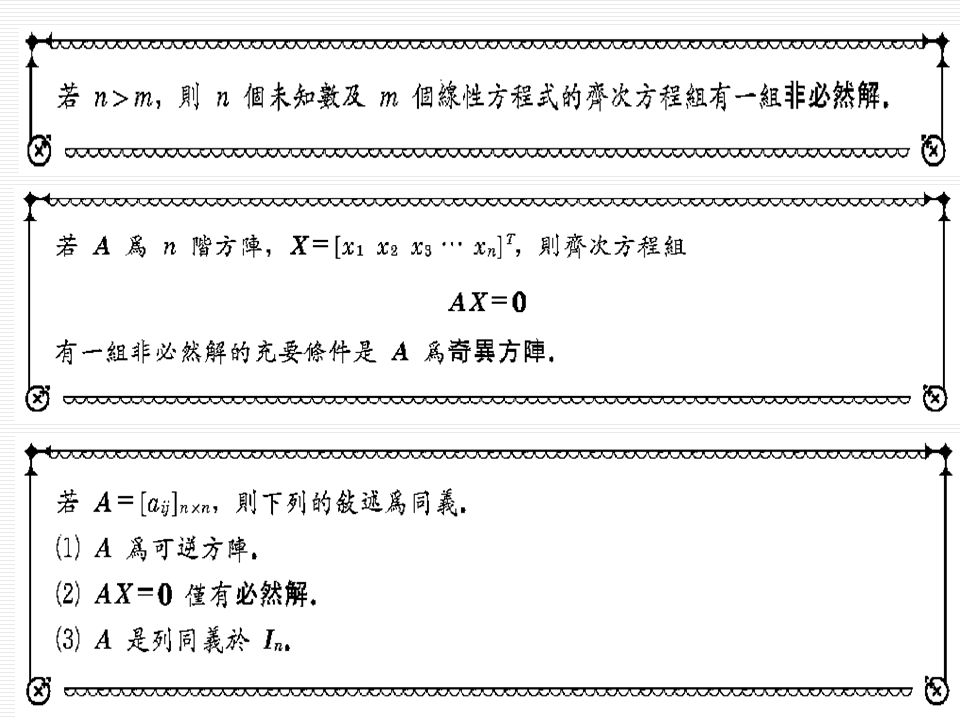
Homogeneous System Equations
AX=b為一線性方程組,若b1=b2=…=bm=0,則稱為齊次方程組(homogeneous) ,以 AX=0表之。 x1=x2=…=xn=0為其中一組解,稱為必然解(trivial solution) 若x1、x2、…xn不全為0,則稱為非必然解(nontrivial solution)
 ,以 AX=0表之。 x1=x2=…=xn=0為其中一組解,稱為必然解(trivial solution) 若x1、x2、…xn不全為0,則稱為非必然解(nontrivial solution)")
17
Example:

18
Example:

20
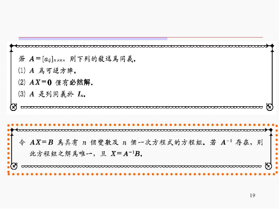
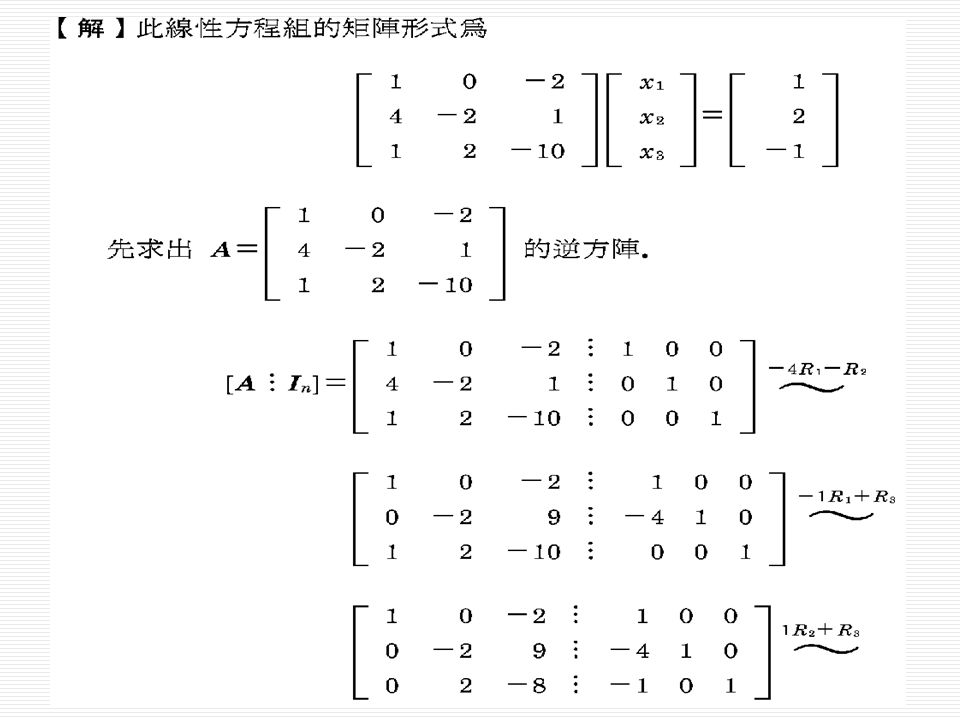
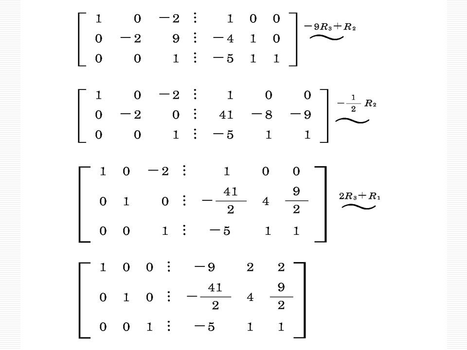
Example : Solving linear system by inverse matrix

24
Exercise : Solving linear system by inverse matrix
(8 min) Answer:
 Answer:")
25
2.6 Determinants(行列式) (p.42)
Associated with any square matrix A is a number called the determinant of A (often abbreviated as det A or |A|). If A is an m x m matrix, then for any values of i and j, the ijth minor of A (written Aij) is the (m - 1) x (m - 1) submatrix of A obtained by deleting row i and column j of A. Determinants can be used to invert square matrices and to solve linear equation systems.
. If A is an m x m matrix, then for any values of i and j, the ijth minor of A (written Aij) is the (m - 1) x (m - 1) submatrix of A obtained by deleting row i and column j of A. Determinants can be used to invert square matrices and to solve linear equation systems.")
26
Determinants(行列式)
")
27
Minor(子行列式) & Cofactor(餘因子)
 & Cofactor(餘因子)")
28
餘因子展開式

29
行列式之性質(1)
")
30
行列式之性質(2)
")
31
行列式之性質(3)
")
32
行列式之性質(4)
")
33
Adjoint matrix (伴隨矩陣)
")
34
Exercise : adj A = ? det(A) = ? Answer: det(A) = -34
 = ? Answer: det(A) = -34")
35
Exercise : 若det(λI3-A)=0, λ=? λ =-5 或λ=0或λ=3
=0, λ=? λ =-5 或λ=0或λ=3")
36
伴隨矩陣之性質

37
行列式之性質

38
Cramer’s Rule

39
Cramer’s Rule 注意事項 若det(A) ≠0,則n元一次方程組為相容方程組, 其唯一解為
若det(A) =det(A1) =det(A2)= …=det(An) =0, 則n元一次方程組為相依方程組,其有無限多組解 若det(A) =0,而det(A1) ≠0 或det(A2) ≠0 ,…, 或det(An) ≠0,則n元一次方程組為矛盾方程組,其 為無解。
 =det(A1) =det(A2)= …=det(An) =0, 則n元一次方程組為相依方程組,其有無限多組解. 若det(A) =0,而det(A1) ≠0 或det(A2) ≠0 ,…, 或det(An) ≠0,則n元一次方程組為矛盾方程組,其 為無解。")
40
Example : Solving Linear System
The system has an infinite number of solutions

41
Exercise : Solving linear system by Cramer’s rule
Answer:

42
LU-Decompositions Factoring the coefficient matrix into a product of a lower and upper triangular matrices. This method is well suited for computers and is the basis for many practical computer programs.

43
Solving linear systems by factoring
Let Ax = b,and coefficient matrix A can be factored into a product of n × n matrices as A = LU, where L is lower triangular and U is upper triangular, then the system Ax = b can be solved by as follows: Step 1. Rewrite Ax = b as LUx = b (1) Step 2. Define a n × 1 new matrix y by Ux = y (2) Step 3. Use (2) to rewrite (1) as Ly = b and solve this system for y. Step 4. Substitude y in(2) and solve for x
 Step 2. Define a n × 1 new matrix y by Ux = y (2) Step 3. Use (2) to rewrite (1) as Ly = b and solve this system for y. Step 4. Substitude y in(2) and solve for x.")
44
Example : Solving linear system by LU decomposition
Step 1. A=LU, Ax=b LUx=b

45
Step 2. Ux=y Step 3. Ly=b Solving y by forward-substitution. y1=1, y2=5, y3=2

46
y1=1, y2=5, y3=2 Step 4. Solving y by backward-substitution.
x1=2, x2=-1, x3=2

47
Doolittle method = Assume that A has a Doolittle factorization A = LU. L:unit lower-△,U:upper-△ = The solution X to the linear system AX = b , is found in three steps: 1. Construct the matrices L and U, if possible. 2. Solve LY = b for Y using forward substitution. 3. Solve UX = Y for X using back substitution.

48
Crout method Assume that A has a Doolittle factorization A = LU. L:lower-△,U:unit upper-△ = The solution X to the linear system AX = b , is found in three steps: 1. Construct the matrices L and U, if possible. 2. Solve LY = b for Y using forward substitution. 3. Solve UX = Y for X using back substitution.

49
Solving Linear Equations (see *.doc)
Gauss backward-substitution 高斯後代法 -- forward-substitution Gauss-Jordan Elimination 高斯約旦消去法 -- reduced row echelon matrix Inversed matrix ─ solve Ax=b as x=A-1b LU method ─ solve Ax=b as LUx=b Cramer's Rule ─ x1=det(A1)/det(A),….
/det(A),….")
Similar presentations


>")


 淡江大學 電機系 翁慶昌 教授 1.1 Introduction to Systems of Linear Equations.>")


>")

>")
