1. Next Generation 802.11n Dina Katabi Jointly with Kate Lin and Shyamnath Gollakota

2. Wireless nodes increasingly have heterogeneous numbers of antennas 1-antenna devices2-antenna devices3-antenna devices

3. 802.11 Was Designed for 1-Antenna Nodes When a single-antenna node transmits, multi-antenna nodes refrain from transmitting Alice Bob Chris

4. But, MIMO Nodes Can Receive Multiple Concurrent Streams Alice Bob Chris

5. Alice It’s Not That Simple But, how do we transmit without interfering at receivers with fewer antennas? Interference!! Bob Chris

6. Enable concurrent transmissions without harming ongoing transmissions Goal 802.11n +

7. Enables 802.11 nodes to contend for both time and concurrent transmissions Maintains random access

8. 1.How to transmit without interfering with receivers with fewer antennas?  Interference nulling  Interference alignment 2.How do we achieve it in a random access manner?  Multi-dimensional carrier sense

9. 1.How to transmit without interfering with receivers with fewer antennas?  Interference nulling  Interference alignment 2.How do we achieve it in a random access manner?  Multi-dimensional carrier sense

10. Interference Nulling Alice Bob nulling Signals cancel each other at Alice’s receiver Signals don’t cancel each other at Bob’s receiver  Because channels are different

11. Interference Nulling Signals cancel each other at Alice’s receiver Signals don’t cancel each other at Bob’s receiver  Because channels are different Bob’s sender learns channels either by feedback from Alice’s receiver or via reciprocity Alice Bob

12. Interference Nulling Q: How to transmit without interfering with receivers with fewer antennas? A: Nulling Q: How to transmit without interfering with receivers with fewer antennas? A: Nulling Alice Bob

13. Alice Bob Chris

14. Is Nulling Alone Enough? NO!! Alice Bob Chris NO!

15. Is Nulling Alone Enough? NO!! Alice Bob Chris NO! Chris needs to null at three antennas

16. Is Nulling Alone Enough? NO!! Alice Bob Chris Transmit Nothing!!! NO! null Are we doomed? No, we can use interference alignment Are we doomed? No, we can use interference alignment

17. MIMO Basics 1.N-antenna node receives in N-dimensional space antenna 1 antenna 2 antenna 1 antenna 2 antenna 3

18. MIMO Basics 1.N-antenna node receives in N-dimensional space 2.N-antenna receiver can decode N signals 2-antenna receiver y1 y2

19. MIMO Basics 1.N-antenna node receives in N-dimensional space 2.N-antenna receiver can decode N signals 3.Transmitter can rotate the received signal y’ y 2-antenna receiver = Ry Rotate by multiplying transmitted signal by a rotation matrix R

20. Interference Alignment wanted signal I1I1 I2I2 If I 1 and I 2 are aligned,  appear as one interferer  2-antenna receiver can decode the wanted signal 2-antenna receiver

21. Interference Alignment If I 1 and I 2 are aligned,  appear as one interferer  2-antenna receiver can decode the wanted signal 2-antenna receiver I 1 + I 2 wanted signal

22. aligning Use Nulling and Alignment nulling Alice (unwanted) Bob Chris Alice Bob Chris Null as before

23. aligning Use Nulling and Alignment Alice Bob Chris nulling Alice + Chris (unwanted) Bob 2-signals in 2D-space  Can decode Bob’s signal

24. Alice Bob Chris Use Nulling and Alignment 3 packets through receivers have fewer than 3 antennas

25. MAC Protocol Each sender computes in a distributed way  where and how to null  where and how to align Analytically proved:  # concurrent streams = # max antenna per sender

26. 1.How to transmit without interfering with ongoing transmissions?  Interference nulling  Interference alignment 2.How do we achieve it in a random access manner?  Multi-dimensional carrier sense

27. 1.How to transmit without interfering with receivers with fewer antennas?  Interference nulling  Interference alignment 2.How do we achieve it in a random access manner?  Multi-dimensional carrier sense

28. Alice Bob Chris Centralized controller

29. But, lost the benefit of 802.11 random access Alice Bob Chris Bob, Chris, both you can transmit a packet concurrently Centralized controller n + maintains random access!

30. In 802.11, contend using carrier sense Multi-Dimensional Carrier Sense But, how to contend despite ongoing transmissions?

31. Alice Bob Alice one signal Alice Bob two signals Say that Ben is performing carrier sense Ben Distinguishable using simple linear algebra

32. Multi-Dimensional Carrier Sense Alice Bob Contend Ben Alice Contend Alice Bob and Ben contend for a second concurrent transmission

33. Multi-Dimensional Carrier Sense Alice Bob Ben Alice Project orthogonal to Alice’s signal Alice Contend

34. Multi-Dimensional Carrier Sense Alice Bob Contend orthogonal to Alice no signal from Alice!! Alice orthogonal to Alice no signal from Alice!! Ben Alice Contend Project orthogonal to Alice’s signal

35. Multi-Dimensional Carrier Sense Alice Bob Alice Apply carrier sense in the orthogonal space Ben Alice orthogonal to Alice no signal from Alice!! orthogonal to Alice no signal from Alice!! Contend

36. Alice Bob Detect energy after projection Multi-Dimensional Carrier Sense Win Lose Ben

37. To contend for the next concurrent transmission Project orthogonal to ongoing signals Apply standard carrier sense Multi-Dimensional Carrier Sense

38. 1.How to transmit without interfering with receivers with fewer antennas?  Interference nulling  Interference alignment 2.How do we achieve it in a random access manner?  Multi-dimensional carrier sense

39. Performance

40. Implementation Implemented in USRP2 OFDM with 802.11-style modulations and convolutional codes

41. Testbed Randomly assign the nodes to the marked locations

42. 1.How to transmit without interfering with ongoing transmissions?  Interference nulling  Interference alignment 2.How do we achieve it in a random access manner?  Multi-dimensional carrier sense

43. 1.How to transmit without interfering with ongoing transmissions?  Interference nulling  Interference alignment 2.How do we achieve it in a random access manner?  Multi-dimensional carrier sense

44. Nulling Experiment wanted signal unwanted signal Can Bob null his signal at Alice’s receiver? Bob Alice

45. 0 Nulling Experiment 802.11 SNR range

46. Nulling Experiment Residual interference from Bob can reduce the SNR of wanted signal by at most ~ 1dB 0

47. Alignment and Nulling Experiment 0

48. Though alignment is harder, residual interference is still small ~1.5dB 0

49. 1.How to transmit without interfering with ongoing transmissions?  Interference nulling  Interference alignment 2.How do we achieve it in a random access manner?  Multi-dimensional carrier sense

50. Carrier Sense Experiment tx1tx1 + tx2tx1tx1 + tx2 Traditional CSCS after projection

51. Carrier Sense Experiment tx1tx1 + tx2tx1tx1 + tx2 Can’t identify Hard to distinguish Traditional CSCS after projection

52. Carrier Sense Experiment Hard to distinguish 9dB jump tx1tx1 + tx2tx1tx1 + tx2 Can identify Can’t identify Traditional CSCS after projection

53. Experiment Alice Bob Chris

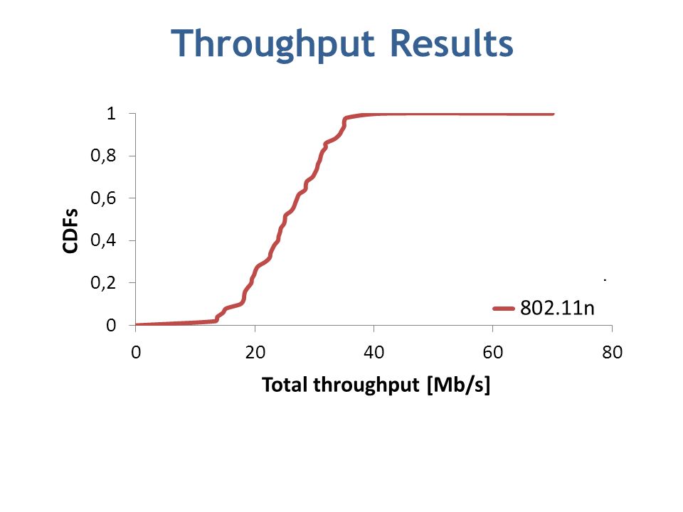
54. Throughput Results

56. ~2x n + doubles the median throughput

57. Related Work Information theory  [CJ08], [MMK08], [JS08], … MIMO systems  Beamforming [AASK10], SAM [TLFWZC09], and IAC [GPK09] N+ is the first random access MAC where nodes contend for time and concurrent transmissions

58. Conclusion In today’s 802.11, MIMO is an add-on In 802.11n +, MIMO is a first-class citizen  Higher concurrency  With random access Shown practical via implementation and testbed evaluation

59. MegaMIMO: Scaling Wireless Throughput with the Number of Users Hariharan Rahul, Swarun Kumar and Dina Katabi

60. Given the trends in the growth of wireless demand, and based on current technology, the FCC projects that the US will face a spectrum shortfall in 2013. The iPhone 4 demo failed at Steve Jobs’s keynote due to wireless congestion. Jobs’s reaction: “If you want to see the demos, shut off your laptops, turn off all these MiFi base stations, and put them on the floor, please.” There is a Looming Wireless Capacity Crunch

61. MegaMIMO MegaMIMO alleviates the capacity crunch by transmitting more bits per unit of spectrum using a distributed MIMO transmitter

62. Access Point 1 Access Point 2 Today’s Wireless Networks Ethernet Access Point 3 User 2 User 3 User 1 Interference! Access Points Can’t Transmit Together in the Same Channel

63. Interference from x 2 +x 3 ≈0 Data: x 1 survives MegaMIMO All Access Points Can Transmit Simultaneously in the Same Channel Interference from x 1 +x 3 ≈0 Data: x 2 survives Interference from x 1 +x 2 ≈0 Data: x 3 survives User 2 User 3 User 1 Access Point 1 Access Point 2 Ethernet Access Point 3 Enables senders to transmit together without interference

64. User 1 Ethernet AP1 User 2 AP2 User 3 AP3 User 10 AP10 … … Distributed protocol for APs to act as a huge MIMO transmitter with sum of antennas 10 APs  10x higher throughput MegaMIMO = Distributed MIMO

65. Diving Into The Details

66. AP 2 AP 1 Cli 1 Cli 2 Wants x 1 Receives y 1 y 1 = d 1 x 1 + 0. x 2 Wants x 2 Receives y 2 y 2 = 0. x 1 + d 2 x 2 y1y1 y2y2 = x1x1 x2x2 d1d1 0 0 d2d2 Transmitting Without Interference

67. AP 2 AP 1 Cli 1 Cli 2 Wants x 1 y 1 = d 1 x 1 + 0. x 2 Wants x 2 y 2 = 0. x 1 + d 2 x 2 y1y1 y2y2 = x1x1 x2x2 D Diagonal Transmitting Without Interference Receives y 1 Receives y 2 Goal: Make the effective channel matrix diagonal Diagonal Matrix  Non-Interference

68. On-Chip MIMO All antennas on the MIMO sender are synchronized in time to within nanoseconds of each other. All antennas on a MIMO sender have exactly the same oscillator, i.e., no frequency offset.

69. y 1 = h 11 x 1 + h 12 x 2 y 2 = h 21 x 1 + h 22 x 2 y1y1 y2y2 = x1x1 x2x2 h 11 h 22 h 12 h 21 On-Chip MIMO Non-diagonal Matrix  Interference AP Cli 1 Cli 2 Sends x 1 Sends x 2 h 11 h 12 h 21 h 22 y1y1 y2y2

70. y 1 = h 11 x 1 + h 12 x 2 y 2 = h 21 x 1 + h 22 x 2 y1y1 y2y2 = x1x1 x2x2 h 11 h 22 h 12 h 21 On-Chip MIMO AP Cli 1 Cli 2 Sends x 1 Sends x 2 h 11 h 12 h 21 h 22 y1y1 y2y2

71. y 1 = h 11 s 1 + h 12 s 2 y 2 = h 21 s 1 + h 22 s 2 y1y1 y2y2 = s1s1 s2s2 h 11 h 22 h 12 h 21 On-Chip MIMO AP Cli 1 Cli 2 Sends s 1 Sends s 2 h 11 h 12 h 21 h 22 y1y1 y2y2

72. y 1 = h 11 s 1 + h 12 s 2 y 2 = h 21 s 1 + h 22 s 2 y1y1 y2y2 = s1s1 s2s2 H On-Chip MIMO AP Cli 1 Cli 2 Sends s 1 Sends s 2 h 11 h 12 h 21 h 22 y1y1 y2y2

73. y 1 = h 11 s 1 + h 12 s 2 y 2 = h 21 s 1 + h 22 s 2 y1y1 y2y2 = s1s1 s2s2 H Making Effective Channel Matrix Diagonal AP Cli 1 Cli 2 Sends s 1 Sends s 2 h 11 h 12 h 21 h 22 y1y1 y2y2

74. y 1 = h 11 s 1 + h 12 s 2 y 2 = h 21 s 1 + h 22 s 2 y1y1 y2y2 = s1s1 s2s2 H Making Effective Channel Matrix Diagonal AP Cli 1 Cli 2 Sends s 1 Sends s 2 h 11 h 12 h 21 h 22 y1y1 y2y2 x1x1 x2x2 H -1

75. y 1 = h 11 s 1 + h 12 s 2 y 2 = h 21 s 1 + h 22 s 2 y1y1 y2y2 = x1x1 x2x2 H H -1 Effective channel is diagonal Making Effective Channel Matrix Diagonal AP Cli 1 Cli 2 Sends s 1 Sends s 2 h 11 h 12 h 21 h 22 y1y1 y2y2

76. MIMO sender computes its beamformed signal s i using the equation Clients 1 and 2 decode x 1 and x 2 independently Measure channels from sending antennas to clients Clients report measured channels back to APs Beamforming System Description Channel Measurement: Data Transmission: s = H -1 x

77. Distributed Transmitters Are Different Nodes are not synchronized in time. – We use SourceSync to synchronize senders within 10s of ns – Works for OFDM based systems like Wi-Fi, LTE etc. Oscillators are not synchronized and have frequency offsets relative to each other.

78. Packet Detection Delay Receivers detect packet using correlation Random noise  Do not detect packet on first sample Different receivers  different noise  different detection delay Peak

79. Packet Detection Delay Receivers detect packet using correlation Random noise  Do not detect packet on first sample Different receivers  different noise  different detection delay Peak

80. Receivers detect packet using correlation Random noise  Do not detect packet on first sample Different receivers  different noise  different detection delay Packet Detection Delay Peak

81. Packet Detection Delay APs estimate packet detection delay Compensate for detection delay by syncing to first sample

82. Estimating Packet Detection Delay OFDM transmits signal over multiple frequencies f1

83. Estimating Packet Detection Delay OFDM transmits signal over multiple frequencies f2 f1 First Sample Detect on first sample  Same phase

84. Estimating Packet Detection Delay OFDM transmits signal over multiple frequencies f2 f1 T Detect after T Frequencies rotate at different speeds

85. Estimating Packet Detection Delay OFDM transmits signal over multiple frequencies f2 f1 T Detect after T Different frequencies exhibit different phases Phase = 2πfT

86. Phase OFDM Frequency f Estimating Packet Detection Delay Slope is 2πT Each AP estimates packet detection delay Estimate uses every symbol in packet  Robust to noise Each AP estimates packet detection delay Estimate uses every symbol in packet  Robust to noise

87. Nodes are not synchronized in time. – We use SourceSync to synchronize senders within 10s of ns – Works for OFDM based systems like Wi-Fi, LTE etc. Oscillators are not synchronized and have frequency offsets relative to each other. Distributed Transmitters Are Different

88. MegaMIMO First wireless network that can scale network throughput with the number of transmitters Algorithm for phase synchronization across multiple independent transmitters Demonstrated in a wireless testbed implementation

89. AP 2 AP 1 Cli 1 Cli 2 h 11 h 12 h 21 h 22 h 21 h 11 h 12 What Happens with Independent Oscillators?

90. AP 2 AP 1 Cli 1 Cli 2 h 11 h 12 h 21 h 22 h 21 h 11 h 12 e j( ω - ω )t T1 R1 ω T1 ω R1 What Happens with Independent Oscillators?

91. AP 2 AP 1 Cli 1 Cli 2 h 11 h 12 h 21 h 22 h 21 h 11 h 12 e j( ω - ω )t T1 R1 ω T1 ω R1 What Happens with Independent Oscillators?

92. AP 2 AP 1 Cli 1 Cli 2 h 11 h 12 h 21 h 22 h 21 h 11 h 12 e j( ω - ω )t T1 R1 e j( ω - ω )t T2 R1 ω T1 ω R1 ω T2 What Happens with Independent Oscillators?

93. AP 2 AP 1 Cli 1 Cli 2 h 11 h 12 h 21 h 22 h 21 h 11 h 12 e j( ω - ω )t T1 R1 e j( ω - ω )t T2 R1 ω T1 ω R1 ω T2 What Happens with Independent Oscillators?

94. AP 2 AP 1 Cli 1 Cli 2 h 11 h 12 h 21 h 22 h 21 h 11 h 12 e j( ω - ω )t T1 R1 e j( ω - ω )t T2 R1 ω T1 ω R1 ω T2 ω R2 e j( ω - ω )t T1 R2 e j( ω - ω )t T2 R2 What Happens with Independent Oscillators?

95. AP 2 AP 1 Cli 1 Cli 2 h 11 h 12 h 21 h 22 h 21 h 11 h 12 e j( ω - ω )t T1 R1 e j( ω - ω )t T2 R1 ω T1 ω R1 ω T2 ω R2 e j( ω - ω )t T1 R2 e j( ω - ω )t T2 R2 What Happens with Independent Oscillators? Time Varying

96. AP 2 AP 1 Cli 1 Cli 2 h 11 h 12 h 21 h 22 ω T1 ω R1 ω T2 ω R2 H(t) Channel is Time Varying

97. s 1 (t) AP 2 AP 1 Cli 1 Cli 2 h 11 h 12 h 21 h 22 ω T1 ω R1 ω T2 ω R2 H(t) y 1 (t) y 2 (t) = s 2 (t) Does Traditional Beamforming Still Work?

98. AP 2 AP 1 Cli 1 Cli 2 h 11 h 12 h 21 h 22 ω T1 ω R1 ω T2 ω R2 H(t) y 1 (t) y 2 (t) = x 1 (t) x 2 (t) H -1 Not Diagonal Does Traditional Beamforming Still Work? Beamforming does not work

99. Challenge Channel is Rapidly Time Varying Relative Channel Phases of Transmitted Signals Changes Rapidly With Time Prevents Beamforming

100. Distributed Phase Synchronization Pick one AP as the lead All other APs are slaves – Imitate the behavior of the lead AP by fixing the rotation of their oscillator relative to the lead. High Level Intuition:

101. h 22 h 21 h 11 h 12 e j( ω - ω )t T1 R1 e j( ω - ω )t T2 R1 e j( ω - ω )t T1 R2 e j( ω - ω )t T2 R2 Decomposing H(t) h 22 h 21 h 11 h 12 e j( ω )t T1 e j( ω )t T2 e j( ω )t T1 e j( ω )t T2 e -j ω t R1 e -j ω t R2 0 0

102. h 22 h 21 h 11 h 12 e j( ω )t T1 e j( ω )t T2 e j( ω )t T1 e j( ω )t T2 e -j ω t R1 e -j ω t R2 0 0 Decomposing H(t)

103. h 22 h 21 h 11 h 12 e -j ω t R1 e -j ω t R2 0 0 Decomposing H(t) e j ω t T1 e j ω t T2 0 0

104. h 22 h 21 h 11 h 12 e -j ω t R1 e -j ω t R2 0 0 Decomposing H(t) e j ω t T1 e j ω t T2 0 0

105. e -j ω t R1 e -j ω t R2 0 0 e j ω t T1 e j ω t T2 0 0 H Decomposing H(t) Diagonal Devices cannot track their own oscillator phases…

106. e -j ω t R1 e -j ω t R2 0 0 e j ω t T1 e j ω t T2 0 0 H Decomposing H(t) e j ω t T1 e -j ω t T1

107. e j( ω - ω )t T1 0 0 H Decomposing H(t) R1 e j( ω - ω )t T1 R2 0 0 e j( ω - ω )t T2 T1 1 R(t)T(t) Depends only on transmitters

108. e j( ω - ω )t T1 0 0 H Decomposing H(t) R1 e j( ω - ω )t T1 R2 0 0 e j( ω - ω )t T2 T1 1 R(t)T(t) H(t) = R(t).H.T(t)

109. Beamforming with Different Oscillators s 1 (t) H(t) y 1 (t) y 2 (t) = s 2 (t) R(t).H.T(t) s 1 (t) s 2 (t) = x 1 (t) x 2 (t) H -1 T(t) -1

110. Beamforming with Different Oscillators H(t) y 1 (t) y 2 (t) = R(t).H.T(t) s 1 (t) s 2 (t) = x 1 (t) x 2 (t) H -1 T(t) -1 x 1 (t) x 2 (t) H -1 T(t) -1 Diagonal

111. Transmitter Compensation T(t) = 0 0 e j( ω - ω )t T2 T1 1

112. Transmitter Compensation T(t) -1 = 0 0 e -j( ω - ω )t T2 T1 1 Slave AP imitates lead by multiplying each sample by oscillator rotation relative to lead Requires only local information  Fully distributed

113. Measuring Phase Offset Multiply frequency offset by elapsed time Requires very accurate estimation of frequency offset – Error of 25 Hz (10 parts per BILLION) changes complete alignment to complete misalignment in 20 ms. Need to keep resynchronizing to avoid error accumulation

114. Resynchronization AP 2 AP 1 Cli 1 Cli 2 h 2 lead h 2 lead (t) = h 2 lead e j( ω - ω )t T2 T1 Directly compute phase at each slave by measuring channel from lead

115. Resynchronization AP 2 AP 1 Sync Data Lead AP: – Prefixes data transmission with synchronization header

116. Resynchronization AP 2 AP 1 Sync Data Slave AP: – Receives Synchronization Header – Corrects for change in channel phase from lead – Transmits data

117. Receiver Compensation H(t) y 1 (t) y 2 (t) = R(t).H.T(t) s 1 (t) s 2 (t)

118. H(t) y 1 (t) y 2 (t) = R(t).H.T(t) x 1 (t) x 2 (t) H -1 T(t) -1 y 1 (t) y 2 (t) = R(t) x 1 (t) x 2 (t) R(t) -1 Receiver Compensation

119. R(t) -1 = e -j( ω - ω )t T1 0 0 R1 e -j( ω - ω )t T1 R2

120. R(t) -1 = Receiver Compensation e -j( ω - ω )t T1 0 0 R1 e -j( ω - ω )t T1 R2 Receiver does what it does today – correct for oscillator offset from lead

121. MegaMIMO Protocol Lead AP and slave AP measure channel matrix H to clients Clients report measured channel to APs Each slave AP measures its channel from lead Each AP computes its beamforming signal as Each slave measures its new channel from lead, and multiplies its beamforming signal by change in channel phase. H -1 x Channel Measurement: Data Transmission:

122. Enhancements Decoupling channel measurement across different clients Using MegaMIMO for diversity Compatibility with off-the-shelf 802.11n cards Described in paper

123. Performance

124. Implementation Implemented in USRP2 2.4 GHz center frequency OFDM with 10 MHz bandwidth 10 software radios acting as APs, all in the same frequency 10 software radios acting as clients

125. Testbed

126. Does MegaMIMO Scale Throughput with the Number of Users? Fix a number of users, say N Pick N AP locations Pick N client locations Vary N from 1 to 10 Compared Schemes: – 802.11 – MegaMIMO

127. Does MegaMIMO Scale Throughput with the Number of Users? Total Throughput [Mb/s] Number of APs on Same Channel

128. Does MegaMIMO Scale Throughput with the Number of Users? 802.11 Total Throughput [Mb/s] Number of APs on Same Channel

129. Does MegaMIMO Scale Throughput with the Number of Users? MegaMIMO 802.11 Total Throughput [Mb/s] Number of APs on Same Channel 10x 10x throughput gain over existing Wi-Fi

130. What are MegaMIMO’s Scaling Limits? Theoretical Practical N log SNR Can Scale Indefinitely with N Errors in H and phase synchronization affect accuracy of beamforming

131. N APs transmit to N users, N = 2.. 10. Perform MegaMIMO as before, but with a zero signal for some client (i.e. null at that client) What are MegaMIMO’s Scaling Limits? Phase Alignment is Accurate  Received signal at noise floor (0 dB) Inaccuracy in Phase Alignment  Received signal higher than noise floor (>0 dB)

132. What are MegaMIMO’s Scaling Limits? Interference to Noise Ratio (dB) Number of APs on Same Channel

133. What are MegaMIMO’s Scaling Limits? Interference to Noise Ratio (dB) Number of APs on Same Channel Interference to Noise Ratio ~1.5 dB at 10 users

134. Compatibility with 802.11n 802.11n over 20 MHz Bandwidth Two 2-antenna USRPs acting as APs Two 2-antenna 802.11n clients Througput gain of MegaMIMO over 802.11n Demonstrates: – Compatibility with 802.11n clients – Compatibility with MIMO APs and clients

135. Compatibility with 802.11n Fraction of Runs Throughput Gain

136. Compatibility with 802.11n Fraction of Runs Throughput Gain 1.8x Median Gain of 1.8x with 2 receivers

137. Related Work Theoretical – Aeron et al., Simeone et al., Ozgur et al. (Distributed and Virtual MIMO) Empirical – DIDO, Fraunhofer – Network MIMO

138. Conclusion Learned about Nulling, Alignment, and MegaMIMO In N+, the gains are lower but – Transmitters need not be connected to the same Ethernet and exchange the packets – No need for phase synchronization In MegaMIMO, the gains are linear with the total number of users – Need high speed Ethernet to connect the transmitters – Need tight phase synchronization between transmitters