1. CSCE 552 Fall 2012 3D Models By Jijun Tang

2. Triangles Fundamental primitive of pipelines  Everything else constructed from them  (except lines and point sprites) Three points define a plane Triangle plane is mapped with data  Textures  Colors “Rasterized” to find pixels to draw

3. Mesh

4. Vertices A vertex is a point in space Plus other attribute data  Colors  Surface normal  Texture coordinates  Whatever data shader programs need Triangles use three vertices  Vertices shared between adjacent triangles

5. Textures Array of texels  Same as pixel, but for a texture  Nominally R,G,B,A but can mean anything 1D, 2D, 3D and “cube map” arrays  2D is by far the most common  Basically just a 2D image bitmap  Often square and power-of-2 in size Cube map - six 2D arrays makes hollow cube  Approximates a hollow sphere of texels  For environmental

6. Texture Example

7. High-Level Organization Gameplay and Rendering Render Objects Render Instances Meshes Skeletons Volume Partitioning

8. Gameplay and Rendering Rendering speed varies according to scene  Some scenes more complex than others  Typically 15-60 frames per second Gameplay is constant speed  Camera view should not change game  In multiplayer, each person has a different view, but there is only one shared game  1 update per second (RTS) to thousands (FPS) Keep the two as separate as possible!

9. Render Objects Description of renderable object type Mesh data (triangles, vertices) Material data (shaders, textures, etc) Skeleton (+rig) for animation Shared by multiple instances

10. Render Instances A single entity in a world References a render object  Decides what the object looks like Position and orientation Lighting state Animation state

11. Meshes Triangles Vertices Single material “Atomic unit of rendering”  Not quite atomic, depending on hardware Single object may have multiple meshes  Each with different shaders, textures, etc  Level-Of-Distance (LOD)

12. LOD Objects have different mesh for different distance from the player The mesh should be simpler if object is faraway Many games have LOD, for example, Microsoft Train Simulator

13. Example (40m, 11370 poly)

14. Example (120m, 3900 poly)

15. Volume Partitioning Cannot draw entire world every frame  Lots of objects – far too slow Need to decide quickly what is visible Partition world into areas Decide which areas are visible Draw things in each visible area Many ways of partitioning the world

16. Volume Partitioning - Portals Nodes joined by portals  Usually a polygon, but can be any shape See if any portal of node is visible If so, draw geometry in node See if portals to other nodes are visible  Check only against visible portal shape  Common to use screen bounding boxes Recurse to other nodes

17. Volume Partitioning – Portals Visible Invisible Not tested Eye View frustum Node Portal Test first two portals ??

18. Volume Partitioning – Portals Visible Invisible Not tested Eye Node Portal Both visible

19. Volume Partitioning – Portals Visible Invisible Not tested Eye Node Portal Mark node visible, test all portals going from node ??

20. Volume Partitioning – Portals Visible Invisible Not tested Eye Node Portal One portal visible, one invisible

21. Volume Partitioning – Portals Visible Invisible Not tested Eye Node Portal Mark node as visible, other node not visited at all. Check all portals in visible node ?? ?

22. Volume Partitioning – Portals Visible Invisible Not tested Eye Node Portal One visible, two invisible

23. Volume Partitioning – Portals Visible Invisible Not tested Eye Node Portal Mark node as visible, check new node’s portals ?

24. Volume Partitioning – Portals Visible Invisible Not tested Eye Node Portal One portal invisible. No more visible nodes or portals to check. Render scene.

25. Real Example

26. Volume Partitioning – Portals Portals are simple and fast Low memory footprint Automatic generation is difficult, and generally need to be placed by hand Hard to find which node a point is in, and must constantly track movement of objects through portals Best at indoor scenes, outside generates too many portals to be efficient

27. Volume Partitioning – BSP Binary space partition tree Tree of nodes Each node has plane that splits it in two child nodes, one on each side of plane Some leaves marked as “solid” Others filled with renderable geometry

28. BSP

29. Volume Partitioning – BSP Finding which node a point is in is fast  Start at top node  Test which side of the plane the point is on  Move to that child node  Stop when leaf node hit Visibility determination is similar to portals  Portals implied from BSP planes Automated BSP generation is common Generates far more nodes than portals  Higher memory requirements

30. Volume Partitioning: Quadtree Quadtree (2D) and octree (3D)  Quadtrees described here  Extension to 3D octree is obvious Each node is square  Usually power-of-two in size Has four child nodes or leaves Each is a quarter of size of parent

31. Quadtree

32. Octree

33. Volume Partitioning - PVS Potentially visible set Based on any existing node system For each node, stores list of which nodes are potentially visible Use list for node that camera is currently in  Ignore any nodes not on that list – not visible Static lists  Precalculated at level authoring time  Ignores current frustum  Cannot deal with moving occluders

34. PVS Room A Room B Room C Room D Room E Viewpoint PVS = B, A, D

35. Volume Partitioning - PVS Very fast  No recursion, no calculations Still need frustum culling Difficult to calculate  Intersection of volumes and portals  Lots of tests – very slow Most useful when combined with other partitioning schemes

36. Rendering Primitives Strips, Lists, Fans Indexed Primitives The Vertex Cache Quads and Point Sprites

37. Strips, Lists, Fans 1 2 3 4 5 6 7 8 9 1 2 3 4 5 6 7 8 1 2 3 4 5 6 1 2 3 4 5 6 1 2 3 4 5 6 Triangle list Triangle fan Triangle strip Line list Line strip

38. Vertex Sharing List has no sharing  Vertex count = triangle count * 3 Strips and fans share adjacent vertices  Vertex count = triangle count + 2  Lower memory  Topology restrictions  Have to break into multiple rendering calls

39. Vertex Counts Using lists duplicates vertices a lot!  Total of 6x number of rendering vertices  Most meshes: tri count = 2x vert count Strips or fans still duplicate vertices  Each strip/fan needs its own set of vertices  More than doubles vertex count Typically 2.5x with good strips  Hard to find optimal strips and fans  Have to submit each as separate rendering call

40. Strips vs. Lists 32 triangles, 25 vertices4 strips, 40 vertices 25 to 40 vertices is 60% extra data!

41. Indexed Primitives Vertices stored in separate array  No duplication of vertices  Called a “vertex buffer” or “vertex array”  3 numbers (int/float/double) per vertex Triangles hold indices, not vertices Index is just an integer  Typically 16 bits (65,536)  Duplicating indices is cheap  Indexes into vertex array

42. Vertex Index Array

43. The Vertex Cache Vertices processed by vertex shader Results used by multiple triangles Avoid re-running shader for each triangle Storing results in video memory is slow So store results in small cache  Requires indexed primitives  Cache typically 16-32 vertices in size, resulted in around 95% efficiency

44. Cache Performance Size and type of cache usually unknown  LRU (least recently used) or FIFO (first in first out) replacement policy  Also odd variants of FIFO policy  Variable cache size according to vertex type Reorder triangles to be cache-friendly  Not the same as finding optimal strips!  Render nearby triangles together  “Fairly good” is easy to achieve  Ideal ordering still a subject for research

45. CSCE 552 Fall 2012 Graphics By Jijun Tang

46. Fundamentals Frame and Back Buffer Visibility and Depth Buffer Triangles Vertices Coordinate Spaces Textures Shaders Materials

47. Frame and Back Buffer Both hold pixel colors Frame buffer is displayed on screen Back buffer is just a region of memory Image is rendered to the back buffer  Half-drawn images are very distracting  You do not want to see the screen is drawn pixel by pixel

48. Two Buffers

49. Switching Back buffer can be standard, frame buffer should aim at each hardware Swapped to the frame buffer  May be a swap, or may be a copy  Copy is actually preferred, because you can still modify the format Back buffer is larger if anti-aliasing  Some hardware may not support anti-aliasing  Shrink and filter to frame buffer

50. Anti-aliasing

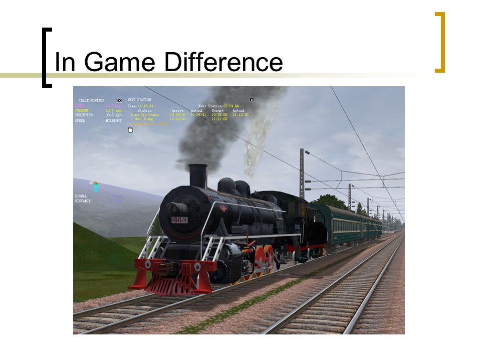
51. In Game Difference

53. Visibility and Depth Buffer Depth buffer is a buffer that holds the depth of each pixel in the scene, and is the same size as back buffer Holds a depth or “Z” value (often called the “Z buffer”) Pixels test their depth against existing value  If greater, new pixel is further than existing pixel  Therefore hidden by existing pixel – rejected  Otherwise, is in front, and therefore visible  Overwrites value in depth buffer and color in back buffer No useful units for the depth value  By convention, nearer means lower value  Non-linear mapping from world space

54. Object Depth Is Difficult

55. Basic Depth Buffer Algorithm for each object in scene in any order for each pixel in the object being rendered if the pixel has already been rendered, then if the new object pixel is closer than the old one, then Replace the displayed pixel with the new one

56. Frustum The viewing frustum is the region of space in the modeled world that may appear on the screen Frustum culling is the process of removing objects that lie completely outside the viewing frustum from the rendering process

57. Frustum and Frustum Culling

58. Coordinate Spaces World space  Arbitrary global game space Object space  Child of world space  Origin at entity’s position and orientation  Vertex positions and normals stored in this Camera space  Camera’s version of “object” space Screen (image) space  Clip space vertices projected to screen space  Actual pixels, ready for rendering

59. Relationship

60. Clip Space Distorted version of camera space Edges of screen make four side planes Near and far planes  Needed to control precision of depth buffer Total of six clipping planes Distorted to make a cube in 4D clip space Makes clipping hardware simpler

61. Clip Space Eye Triangles will be clipped Camera space visible frustum Clip space frustum

62. Shaders A program run at each vertex or pixel  Generates pixel colors or vertex positions Relatively small programs  Usually tens or hundreds of instructions Explicit parallelism  No direct communication between shaders  “Extreme SIMD” programming model Hardware capabilities evolving rapidly

63. Example

64. Textures Texture Formats Texture Mapping Texture Filtering Rendering to Textures

65. Textures Array of texels  Same as pixel, but for a texture  Nominally R,G,B,A but can mean anything 1D, 2D, 3D and “cube map” arrays  2D is by far the most common  Basically just a 2D image bitmap  Often square and power-of-2 in size Cube map - six 2D arrays makes hollow cube  Approximates a hollow sphere of texels  For environmental

66. Texture Example

67. Texture Formats Textures made of texels Texels have R,G,B,A components  Often do mean red, green, blue colors  Really just a labelling convention  Shader decides what the numbers “mean” Not all formats have all components Different formats have different bit widths for components  Trade off storage space and speed for fidelity  Accuracy concerns

68. Common formats A8R8G8B8 (RGBA8):  32-bit RGB with Alpha  8 bits per comp, 32 bits total R5G6B5: 5 or 6 bits per comp, 16 bits total A32f: single 32-bit floating-point comp A16R16G16B16f: four 16-bit floats DXT1: compressed 4x4 RGB block  64 bits  Storing 16 input pixels in 64 bits of output (4 bits per pixel)  Consisting of two 16-bit R5G6B5 color values and a 4x4 two bit lookup table

69. Texels Arrangement Texels arranged in variety of ways  1D linear array of texels  2D rectangle/square of texels  3D solid cube of texels  Six 2D squares of texels in hollow cube All the above can have mipmap chains  Mipmap is half the size in each dimension  Mipmap chain – all mipmaps to size 1

70. MIP Maps Pre-calculated, optimized collections of bitmap images that accompany a main texture MIP meaning "much in a small space“ Each bitmap image is a version of the main texture, but at a certain reduced level of detail (like LOD in 3D Models)

71. MIPMapping Example

72. Texture Mapping Texture coordinates called U, V, W Only need U for 1D; U,V for 2D U,V,W typically stored in vertices Or can be computed by shaders Ranges from 0 to 1 across texture  No matter how many texels the texture contains (64X64, 128X128, etc)  Except for cube map – range is -1 to +1

73. Texture Example