1. Chapter 11 HYPOTHESIS TESTING USING THE ONE-WAY ANALYSIS OF VARIANCE

2. Moving Forward Your goals in this chapter are to learn: The terminology of analysis of variance When and how to compute Why should equal 1 if H 0 is true, and why it is greater than 1 if H 0 is false When and how to compute Tukey’s HSD How eta squared describes effect size

3. Analysis of Variance The analysis of variance is the parametric procedure for determining whether significant differences occur in an experiment with two or more sample means In an experiment involving only two conditions of the independent variable, you may use either a t-test or the ANOVA

4. An Overview of ANOVA

5. One-Way ANOVA Analysis of variance is abbreviated as ANOVA An independent variable is also called a factor Each condition of the independent variable is called a level or treatment Differences produced by the independent variable are a treatment effect

6. Between-Subjects A one-way ANOVA is performed when one independent variable is tested in the experiment When an independent variable is studied using independent samples in all conditions, it is called a between-subjects factor A between-subjects factor involves using the formulas for a between-subjects ANOVA

7. Within-Subjects Factor When a factor is studied using related (dependent) samples in all levels, it is called a within-subjects factor This involves a set of formulas called a within- subjects ANOVA

8. Diagram of a Study Having Three Levels of One Factor

9. Assumptions of the ANOVA 1.All conditions contain independent samples 2.The dependent scores are normally distributed, interval or ratio scores 3.The variances of the populations are homogeneous

10. Experiment-Wise Error The probability of making a Type I error somewhere among the comparisons in an experiment is called the experiment-wise error rate When we use a t-test to compare only two means in an experiment, the experiment-wise error rate equals 

11. Comparing Means When there are more than two means in an experiment, the multiple t-tests result in an experiment-wise error rate much larger than the  we have selected Using the ANOVA allows us to make all our decisions and keep the experiment-wise error rate equal to 

12. Statistical Hypotheses

13. The F-Test The statistic for the ANOVA is F When F obt is significant, it indicates only that somewhere among the means at least two of them differ significantly It does NOT indicate which specific means differ significantly When the F-test is significant, we perform post hoc comparisons

14. Post Hoc Comparisons Post hoc comparisons are like t-tests We compare all possible pairs of level means from a factor, one pair at a time to determine which means differ significantly from each other

15. Components of the ANOVA

16. Mean Squares The mean square within groups describes the variability in scores within the conditions of an experiment. It is symbolized by MS wn. The mean square between groups describes the differences between the means of the conditions in a factor. It is symbolized by MS bn.

17. The F-Ratio The F-ratio equals the mean square between groups divided by the mean square within groups When H 0 is true, F obt should equal 1 When H 0 is false, F obt should be greater than 1

18. Performing the ANOVA

19. Sum of Squares The computations for the ANOVA require the use of several sums of squared deviations The sum of squares is the sum of the squared deviations of a set of scores around the mean of those scores It is symbolized by SS

20. Summary Table of a One-way ANOVA

21. Computing F obt 1.Compute the sums and means for each level. Add the from all levels to get. Add together the from all levels to get. Add the ns together to get N.

22. Computing F obt 2.Compute the total sum of squares (SS tot )

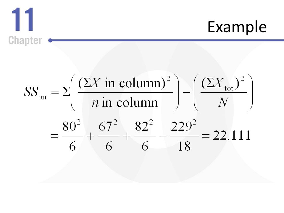
23. Computing F obt 3.Compute the sum of squares between groups (SS bn )

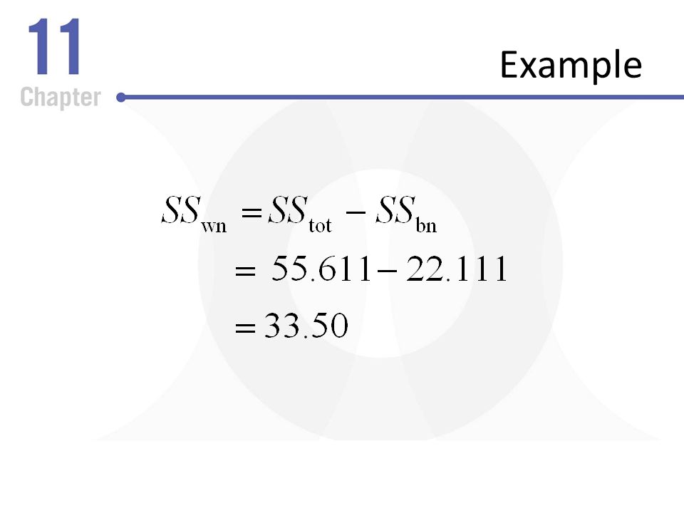
24. Computing F obt 4.Compute the sum of squares within groups (SS wn )

25. Computing F obt Compute the degrees of freedom The degrees of freedom between groups equals k – 1 where k is the number of levels in the factor The degrees of freedom within groups equals N – k The degrees of freedom total equals N – 1

26. Computing F obt Compute the mean squares

27. Computing F obt Compute F obt

28. Sampling Distribution of F When H 0 Is True

29. Degrees of Freedom The critical value of F (F crit ) depends on The degrees of freedom (both the df bn = k – 1 and the df wn = N – k) The  selected The F-test is always a one-tailed test

30. Tukey’s HSD Test When the ns in all levels of the factor are equal, use the Tukey HSD multiple comparisons test where q k is found using Table 5 in Appendix B

31. Tukey’s HSD Test Determine the difference between each pair of means Compare each difference between the means to the HSD If the absolute difference between two means is greater than the HSD, then these means differ significantly

32. Effect Size and Eta 2

33. Proportion of Variance Accounted For Eta squared indicates the proportion of variance in the dependent variable scores that is accounted for by changing the levels of a factor

34. Example Using the following data set, conduct a one-way ANOVA. Use  = 0.05. Group 1 Group 2 Group 3 14 10131115 131012111413 141511101415

35. Example

38. df bn = k – 1 = 3 – 1 = 2 df wn = N – k = 18 – 3 = 15 df tot = N – 1 = 18 – 1 = 17

39. Example

40. F crit for 2 and 15 degrees of freedom and  = 0.05 is 3.68 Since F obt = 4.951, the ANOVA is significant A post hoc test must now be performed

41. Example

42. Because 2.50 > 2.242 (HSD), the mean of sample 3 is significantly different from the mean of sample 2.