Download presentation
Presentation is loading. Please wait.

1
Shape from Contour Recover 3D information

2
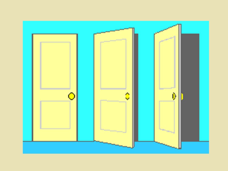
Muller-Lyer illusion

3
Linear perspective - Ponzo illusion

6
Shape 1.Shape is a stable property of objects 2.The difficulty lies in finding a representation of global shape that is general enough to deal with the wide variety of objects in the real world 3.Its most significant role is in object recognition, where geometric shape along with colour and texture provide the most significant cue to enable us to identify objects, classify what is in the image as an example of some class one has seen before

7
Shape from Contour After edge detection, an important question in visual recovery is to deduce the 3-D structure of scene from its line drawing. an inherent ambiguity exists because under perspective projection the line drawing of any scene event, for example, a depth discontinuity, can restrict the location of the event only to a narrow cone of rays (C1)
.")
8
figure C1 - An infinite number of 3D drawings can give rise to the same image The goal of the shape-from-contour module is to derive information about the orientation of the various different faces.

9
A line drawing of a scene consisting of polyhedra. Shaded surfaces are shadows

10
reference Winston, Patrick (1992) Artificial Intelligence (3 rd Edition), Reading (Mass): Addison-Wesley Pub. Co Chapter 12; pp249-272

11
Symbolic Constraints and Propagation Ambiguities – multi-interpretations for an individual components of an input – Enormous possible combinations of the components Some of them may not occur The use of constraints – To reduce the complexity Analyse the problem domain to determine what the constraints are Apply a constraint satisfaction algorithm

12
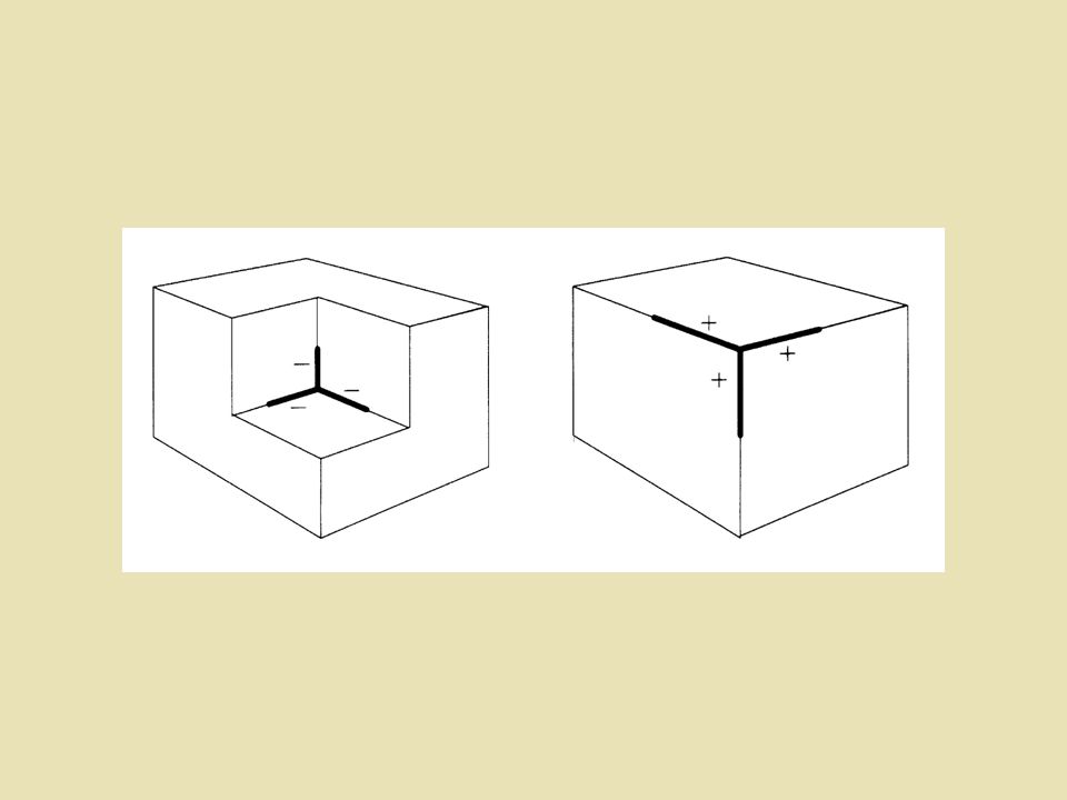
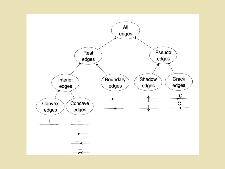
Edges An Obscuring Edge – A boundary between objects, or between object and the background A Concave Edge - An Edge between two faces that form an acute angle when viewed from the outside of the object A Convex Edge – An edge between two faces that form an obtuse angle when viewed from outside the object.

13
The Scope of Lines At moment, not consider cracks between coplanar faces and shadow edge between shadows and the background But the approach is extensible to handle these other types we consider only figures composed exclusively of trihedral vertices, which are vertices at which exactly three planes come together. (figure S1) You need to know this assumption
 You need to know this assumption.")
14
Some trihedral figures Figure S1 - Some trihedral figures

15
figure S1 - Some Nontrihedral figures

16
Determining the Constraints how to recognize individual objects in a figure - our objective to label all the lines in the figure so that we know which ones correspond to boundaries between objects a set of four labels that can be attached to a give line. (S2)
.")
17
Figure S2 - Line labelling conventions + convex line - concave line > Boundary line with interiors to the right (down) < Boundary line with interiors to the right (up)
 < Boundary line with interiors to the right (up)")
18
Figure S2 - An example of line labelling

19
Four Trihedral Vertex Types the number of ways of labeling a figure composed of N lines is 4 N – how to find the correct one? the number of possible line labellings would be reduced, if – constrains on the kinds of vertices – constrains on the lines – every line must meet other lines at a vertex at each of its ends. For the trihedral figures there are only four configurations that describe all the possible vertices. (Figure S3)
.")
20
The four trihedral vertex types (S3)
")
21
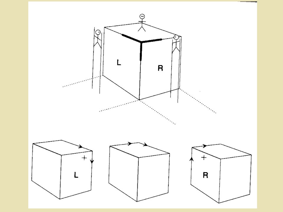
Labels and Their Constraints the maximum number of ways that each of the four types of lines might combine with other lines at a vertex there are 208 ways to form a trihedral vertex But, in fact, only a very small number of these labelings can actually occur in line drawings representing real physical objects (S4)
")
23
A figure occupying one octant (S4)
")
24
S5

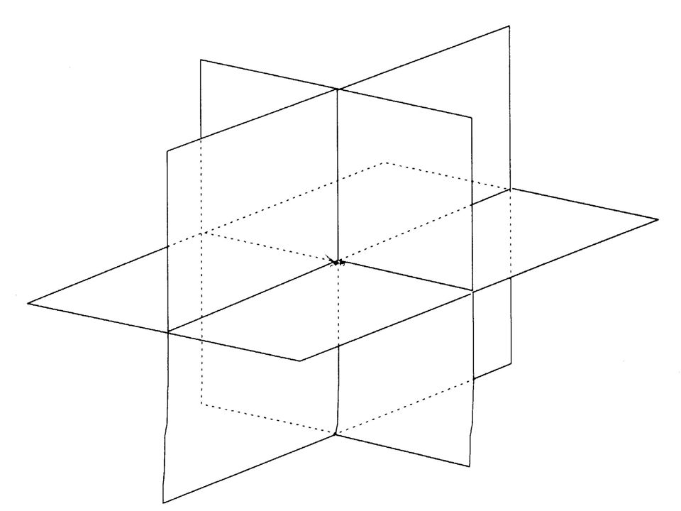
30
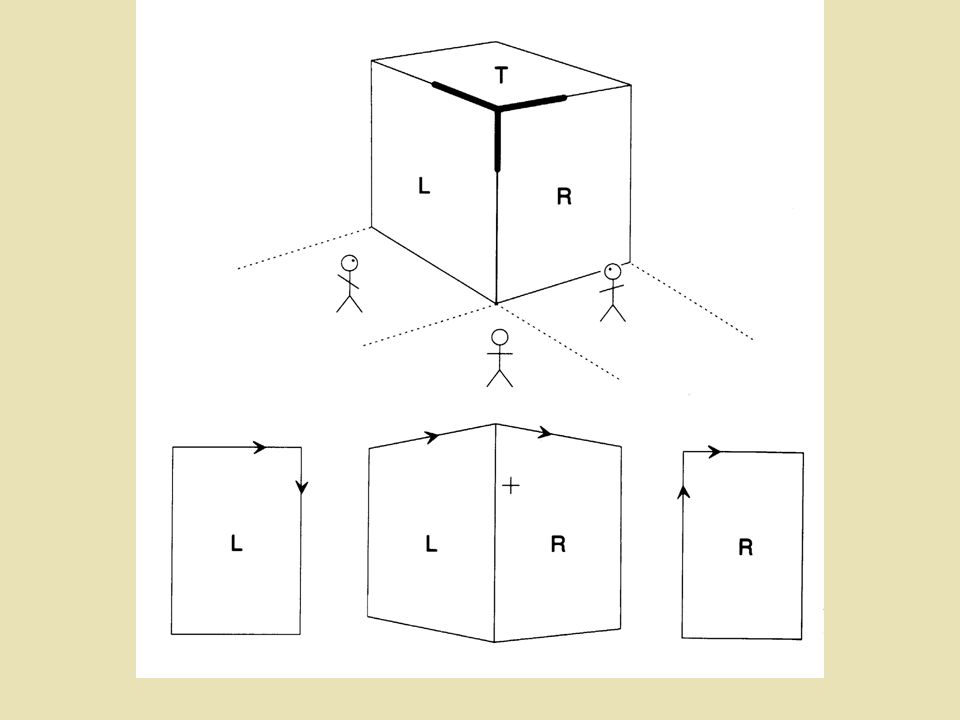
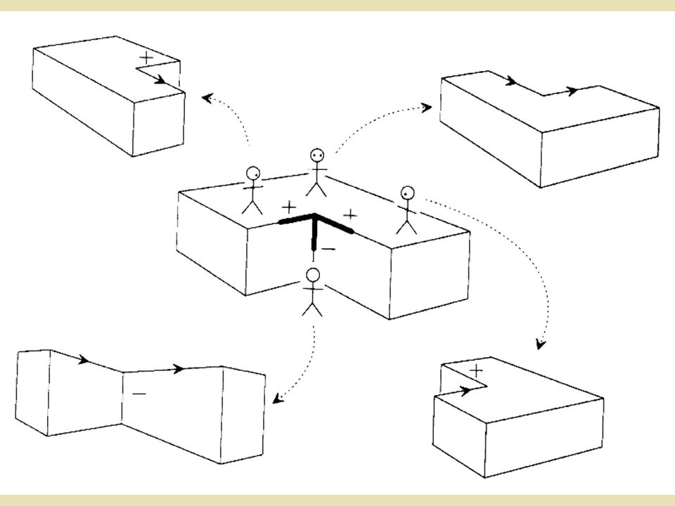
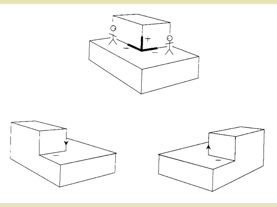
Illustration example Octants – Trihedral figure may differ in the number of octants that they fill and in the position (which must be one of the unfilled octants) from which they are viewed – Any vertex that can occur in a trihedral figure must correspond to such a division of space with some number (between one and eight) of octants filled, which is viewed from one of the unfilled octants So to find all the vertex labelling that can occur, we need only consider all the ways of filling the octants and each of the ways of viewing those fillings, and then record the types of the vertices that we find.
 from which they are viewed – Any vertex that can occur in a trihedral figure must correspond to such a division of space with some number (between one and eight) of octants filled, which is viewed from one of the unfilled octants So to find all the vertex labelling that can occur, we need only consider all the ways of filling the octants and each of the ways of viewing those fillings, and then record the types of the vertices that we find.")
31
Possible Trihedral Vertex Labelings(S5) we get a complete list of the possible trihedral vertices and their labellings (figure S6) the 208 labellings that were theoretically possible, only 18 are physically possible. a severe constraint on the way that lines in drawings corresponding to real figures can be labeled.

32
S6 Label set (18)
")
33
Label set (16)
")
34
W1

35
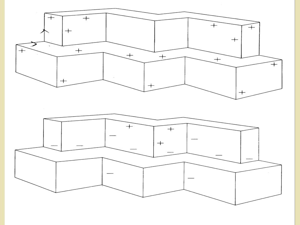
Waltz Procedure 1.pick one vertex and find all the labellings that are possible for it. 2.move to an adjacent vertex and find all of its possible labellings. The line from the first vertex to the second must end up with only one label, and that label must be consistent with the two vertices it enters. 3.inconsistent ones can be eliminated. 4.Continue with another adjacent vertex. Constraints arises from this labelling and these constraints can be propagated back to vertices that have already been labelled, so the set of possible labellings for them is further reduced. 5.This process proceeds until all the vertices in the figure have been labelled. (figure W1, W12)
.")
36
W12

37
Convergent Intelligence Thus symbolic constraint propagation offers a plausible explanation for one kind of human information processing, as well as a good way for computer to analyse drawings. This idea suggest the following principle: The world manifests constraints and regularities. If a computer is to exhibit intelligence, it must exploit those constraints and regularities, no matter of what the computer happens to be made.

38
W12

39
Waltz algorithm Please see the algorithm in the extra note (the handout in class or download from the module website) This algorithm will always find the unique, correct figure labeling if one exists. If a figure is ambiguous, however, the algorithm will terminate with at least one vertex still having more than one labeling attached to it. was applied to a larger class of figures in which cracks and shadows might occur. the usefulness of the algorithm increases as the size of the domain increases and thus the ratio of physically possible to the theoretically possible vertices decreases.

40
W10

42
W11

43
A Sample Example of the Labelling Process

44
Static Constraints and Dynamic Constrains Static constrains: – do not need to be represented explicitly as part of a problem state. – They can be encoded directly into the line- labeling algorithm. dynamic constrains – describe the current options for the labeling of each vertex. – will be represented and manipulated explicitly by the line-labeling algorithm.

45
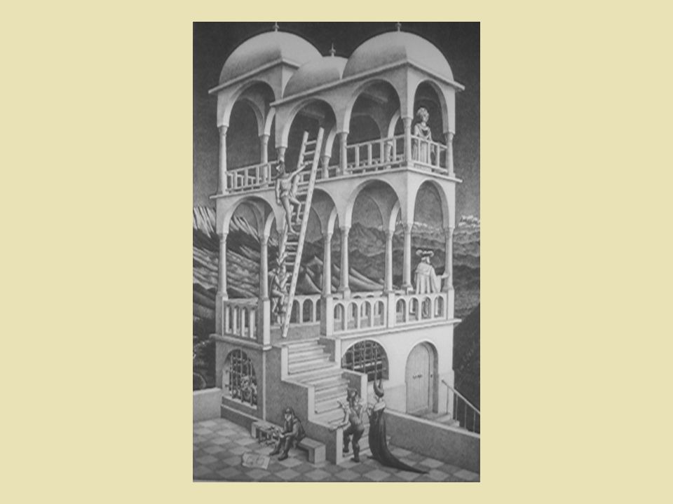
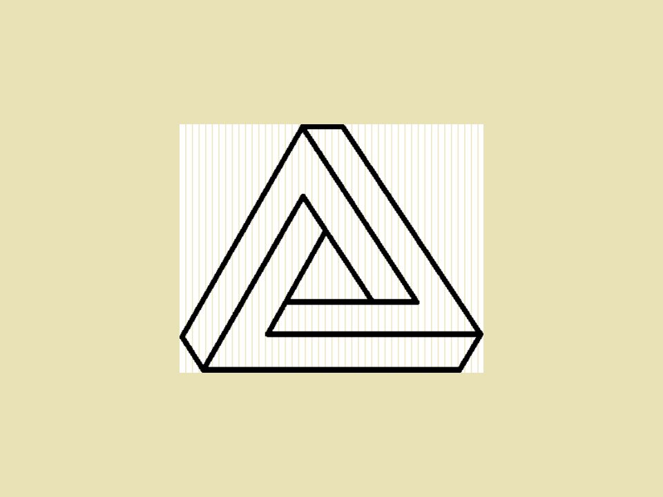
Labelling and Reality Successful labeling is a necessary condition for realizability as an object in trihedral vertex world, but not in a world that allows vertexes with more than three faces. Successful labeling is not a sufficient condition for realizability as an object in a three-faced vertex world (M C Escher, local and global)
.")
48
Extensibility Shadow areas can be of great use in analyzing the scene that is being portrayed When these variations are considered, there become more than eighteen allowable vertex labelings But the ratio of physical allowable vertices to theoretically possible ones becomes even smaller than 18/208. Thus this approach can be extended to larger domains

49
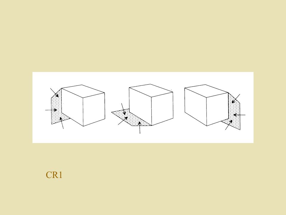
Many lines and junction labels are needed to handle shadows and cracks Shadows help determine where an object rests against others (Cr1) Concave edges often occur where two or three objects meet. It is useful to distinguish among the possibilities by combining the minus label with the one or two boundary labels that are seen when the objects are separated (Cr2)
.")
50
CR1

52
CR2

54
Illumination Increase Label Count and Tightens Constraint There are now 11 ways that any particular line may be labelled 3 2 =9 illumination combinations for each of the 11 line, giving 99 total possibilities. (Cr3) Only 50 of these combinations are possible.
 Only 50 of these combinations are possible..")
55
CR3

56
Summary Understand the major difficulties that confront programs designed to perform perceptual tasks describe the use of constraint satisfaction procedure as one way of surmounting some of those difficulties. perceptual abilities are essential in the the construction of intelligent robots/systems

Similar presentations


Contours 2)Objects 3)Faces 4)Scenes.>")


 A (potential) application of singularity theory to vision BIRS, Banff, 30 August 2011.>")


 l Human Vision l Image Processing l Edge Detection l Convolution and the Canny Edge Detector l.>")
 S. Tanimoto, 2007 Segmentation and Labeling 1 Segmentation and Labeling Outline: Edge detection Chain coding of curves Segmentation into.>")

