1. Ladies Professional Golf Association Winnings (LPGA) VS Senior Professional Golf Association Winnings (SPGA) 2-Sample t-Test

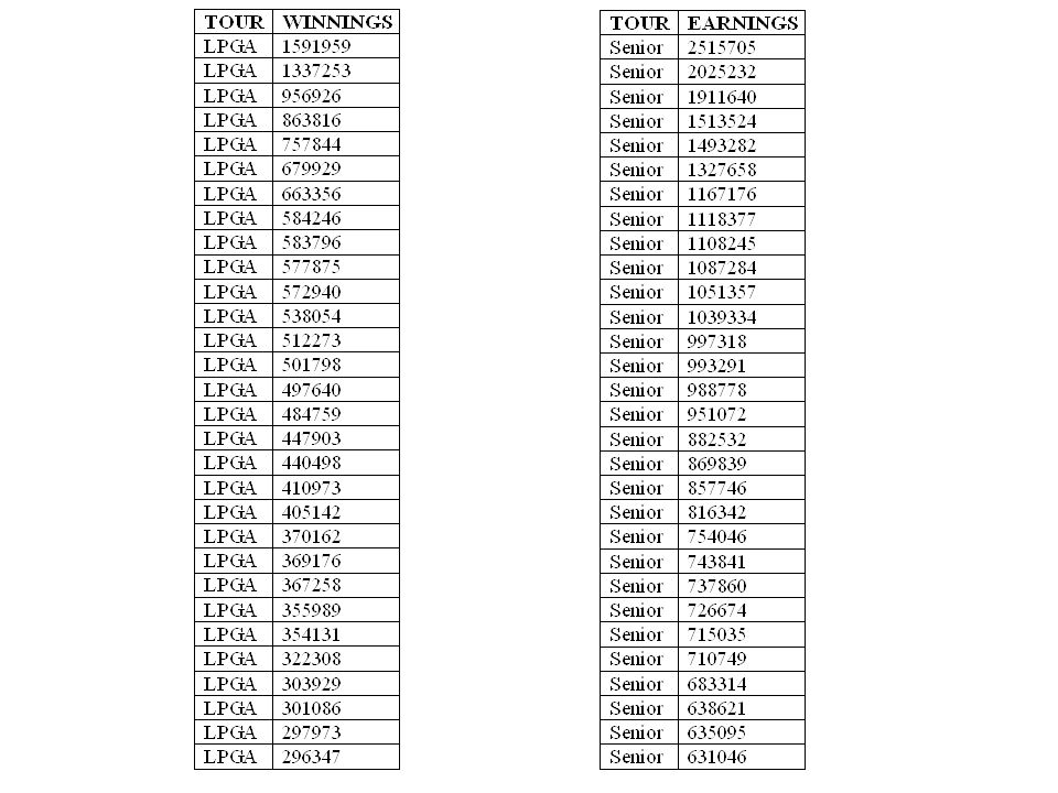
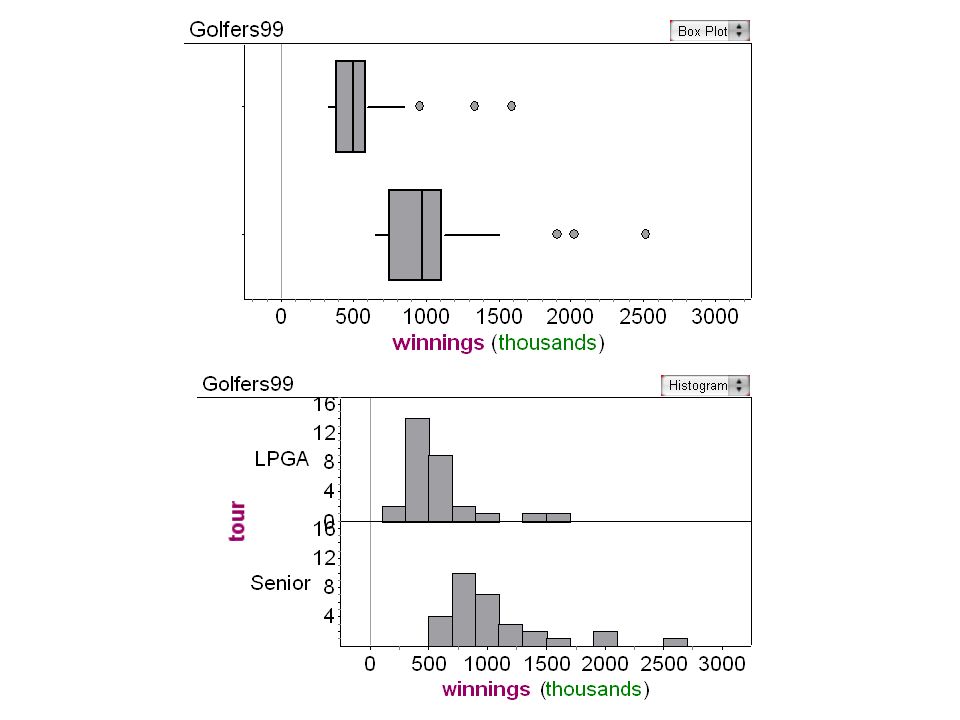
4. MINQ1MEDQ3MAX LPGA2963473672584912005842461591959 SPGA63104673786096992511183772515705 MEANSD LPGA558245299096 SPGA1056400446668 We can see from the graph and the relationships between the mean and median for each data set (mean>median), that both data sets are skewed right. SPGA has a larger center than LPGA. This can be seen from the graphs an comparing the median and mean for each data set. SPGA has a larger spread than LPGA. Both data set have outliers on the high end of the data.

5. Even Though Both graphs are skewed right combined sample size is equal to 60. This was not a random sample since I gathered the top 30 for each tour so this might cause a problem with conclusion. I will Reject H o because p 1.675. My data is statistically significant and I am able to conclude that average winnings on LPGA tour are less than average winning for SPGA tour. Since this was a Reject H o conclusion it is possible that we have committed a Type I Error which would be concluding that the average LPGA winnings is less than SPGA, when in reality the average LPGA winnings are not less than SPGA.

6. The 90% confidence interval for the difference in average winnings(LPGA - SPGA) is (-66000,-33000). Since all the values are negative we can conclude that average winning for LPGA is less than average wining for SPGA

7. Husband’s Age VS Wife’s Ages Matched Pair t-Test

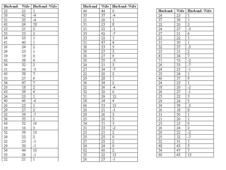
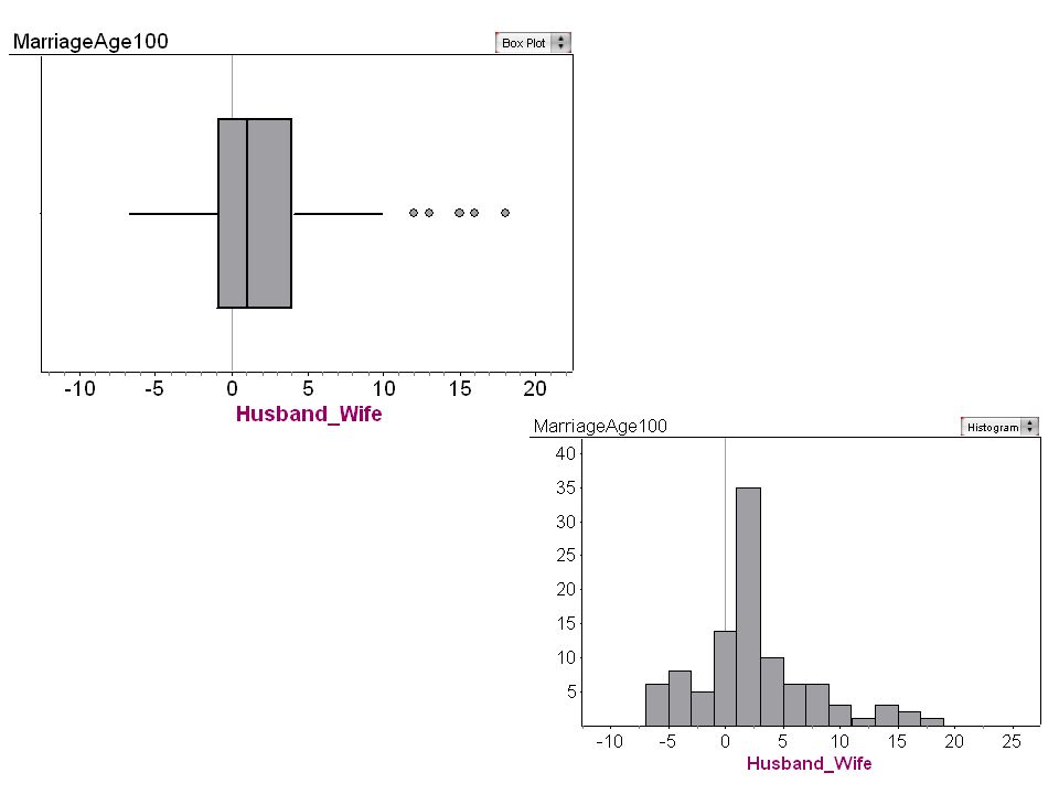
10. MINQ1MEDQ3MAX Husband-Wife-71418 MEANSD Husband-Wife1.925.04661 We can see from the graph and the relationships between the mean and median for each data set (mean>median), that the data sets is skewed right. We can also see that there are outliers on the high end of the data set.

11. Even though the graph is slightly skewed right tah sample size was 100. The data is a SRS I will Reject H o because p 1.66. My data is statistically significant and I am able to conclude that average Husband’s age is greater than average Husband’s are older than their Wife’s age Since this was a Reject H o conclusion it is possible that we have committed a Type I Error which would be concluding that the average Husband age is greater than the average age of their Wife’s, when in reality the average age of a Husband is not greater than the average age of their Wife’s

12. The 90% confidence interval for the average difference in ages(Husband-Wife) is (1.0821,2.7579). Since all the values are positive we can conclude that average Husband’s age is greater than the average Wife’s age

13. Football Injuries VS Baseball Injuries 2-Propotion z-Test

14. SportInjuriesParticipantsProportion Football334420201000000.01664 Baseball326714304000000.01075

15. I will Reject H o because p 1.645. My data is statistically significant and I am able to conclude that a higher proportion of Football players get injured Since this was a Reject H o conclusion it is possible that we have committed a Type I Error which would be concluding a higher proportion of Football players get injured when in reality it is not true that a higher proportion of Football players get injured It is reasonable to assume SRS 20100000(0.01664)>10 20100000(1-0.01664)>10 30400000(0.01075)>10 30400000(1-0.01075)>10

16. The 90% confidence interval for the difference in proportion of injuries (Football - Baseball) is (0.00583,0.00595). Since all the values are positive we can conclude that proportion of Football players who get injured is greater than the proportion of Baseball players who get injured

17. Spending Money For Space Exploration VS Political Perspective Chi-Squared Test for Independence

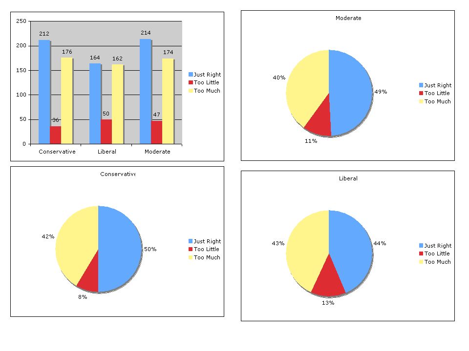
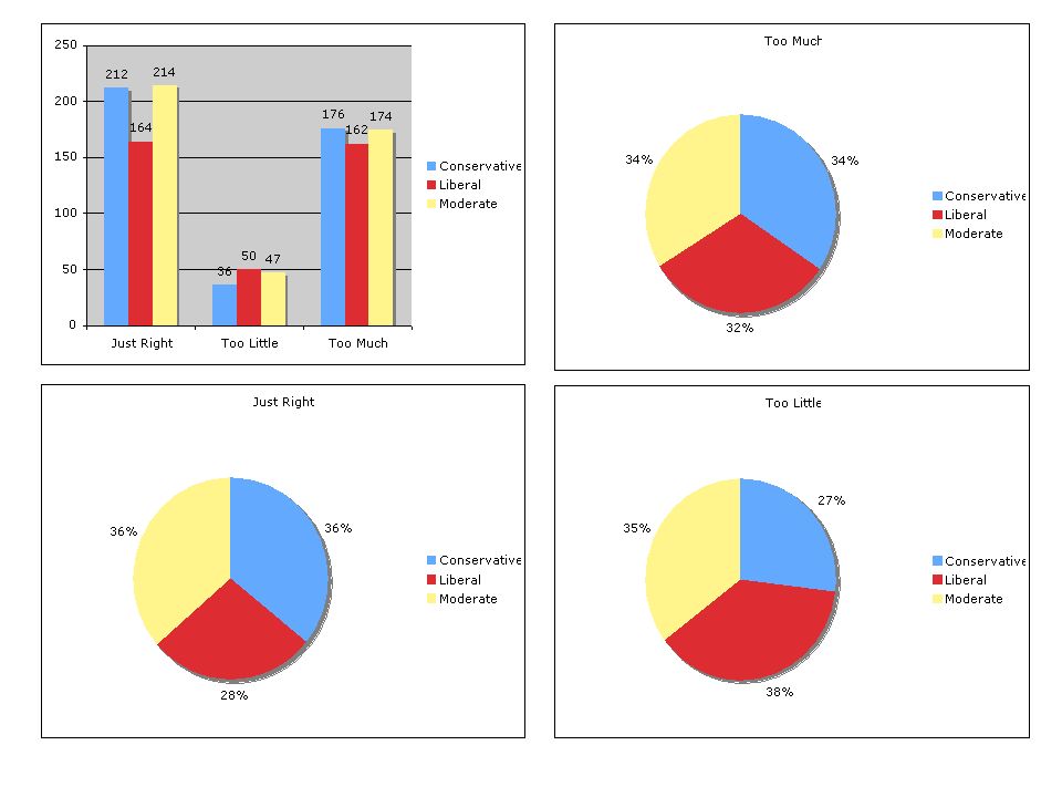
18. ConservativeLiberalModerate Just Right 212164214 Too Little 365047 Too Much 176162174

21. ConservativeLiberalModerate Just Right 202.6179.6207.8 Too Little 45.740.546.8 Too Much 175.8155.9180.3 It is reasonable to assume a SRS and all expected counts are greater than 5

22. I will Fail to Reject H o because p > 0.05 and < 9.49. My data is not statistically significant and I am unable to conclude that there is a relationship between spending perspective and political perspective Since this was a Fail to Reject H o conclusion it is possible that we have committed a Type II Error which would be concluding that there is no relationship between spending perspective and political perspective when in fact a relationship exist

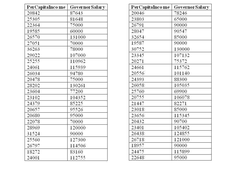
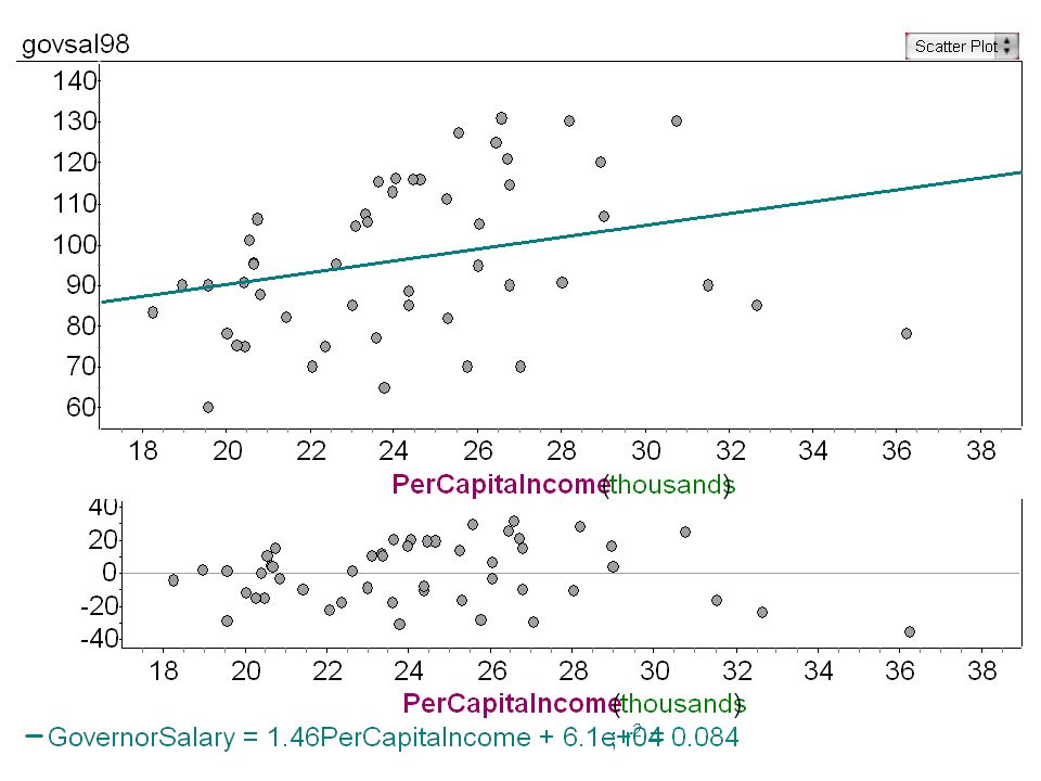
23. Per Capita Income VS Governor's Salary Linear Regression t-Test

26. Te scatter plot and r 2 value indicate a weak linear fit. The residual plot shows an unequal spread of the residual values. These fact could result in incorrect results with test. I will Reject H o because p 1.677. My data is statistically significant and I am able to conclude there is a linear relationship between Per Capita Income and Governor's Salary Since this was a Reject H o conclusion it is possible that we have committed a Type I Error which would be concluding that there is a linear relationship between Per Capita Income and Governor's Salary when no relationship exist

27. The 90% confidence interval for the slope of the line of best fit for Per Capita Income vs. Governor's Salary is (0.2936,2.62032) Since all the values are positive we can conclude that there is a positive relationship between Per Capita Income vs. Governor's Salary