1. Top-points in Image Matching Bram Platel Evgenya Balmashnova Luc Florack Bart ter Haar Romeny

2. Introduction Question: can top-points be used for object-retrieval tasks?

3. Introduction to Scale Space and Deep Structure

4. Importance of Scale in Image Analysis Painting by Dali Objects in images exist at different ranges of scale. Usually it is not known a priory at what scale to look.

5. At the original scale of a dithered image we cannot calculate a derivative. We need to observe the image at a certain scale. BLUR

6. Solution? Look at all scales simultaneously Scale x y Scale Space

7. Scale Space in Human Vision The human visual system is a multi-scale sampling device The retina contains receptive fields; groups of receptors assembled in such a way that they form a set of apertures of widely varying size.

8. Practical Implementation Convolve the image with a Gaussian Kernel

9. We can Calculate Derivatives and Combinations of them at all Scales Gradient Magnitude Laplacian Original Image

10. Main Topic In this presentation we will show how we can exploit the deep structure of images to define invariant interest points and features which can be used for matching problems in computer vision. We consider only grey-value images.

11. Interest Points The locations of particularly characteristic points are called the interest points or key points. These interest points have to be as invariant as possible, but at the same time they have to carry a lot of distinctive information.

12. Why Interest Points in Scale Space? Information in interest points is defined by their neighborhood. But how big should we choose this neighborhood? Let’s take the corners of the mouth as interest points. The red circles are the areas in which the information is gathered. If we make the picture bigger, the size of the neighborhood is too small. The neighborhood should scale with the image

13. Why Interest Points in Scale Space? When the interest points are detected in scale space they do not only have spatial coordinates x and y, but also a scale . This scale tells us how big the neighborhood should be.  

14. Which Interest Points to Use? Our interest points have to be detected in scale space. They also have to… –…contain a lot of information –…be reproducible –…be stable –…be well understood

15. We Suggest Top-Points The points we introduce have these desired properties.

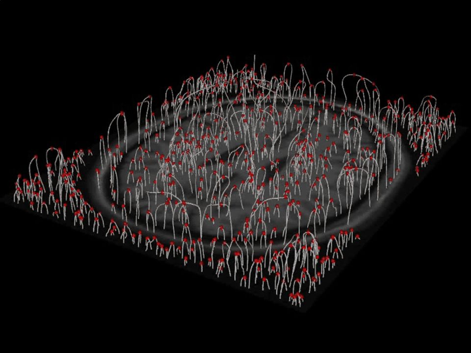
16. Critical Points, Paths and Top-Points Maxima Minimum Saddles  L=0 Critical Points

17. Critical Points, Paths and Top-Points Maxima Minimum Saddles  L=0 Critical Points Det(H)=0 Top-Points

18. Possible to calculate them for every Function of the Image L(x,y,  ) OriginalGradient Magnitude LaplacianDet(H)

19. Detecting Critical Paths Since for a critical path  L=0 Intersection of Level Surfaces L x =0 with L y =0 Will give the critical paths.

20. Detecting Top-Points Since for a top-point both  L=0 and Det[H]=Lxx Lyy- Lxy 2 =0 We can find them by intersecting the paths with the level surface Det[H]=0

22. Invariance of Top Points Top-points are invariant to certain transformations. By invariant we mean that they move according to the transformation. Allowed Trans.

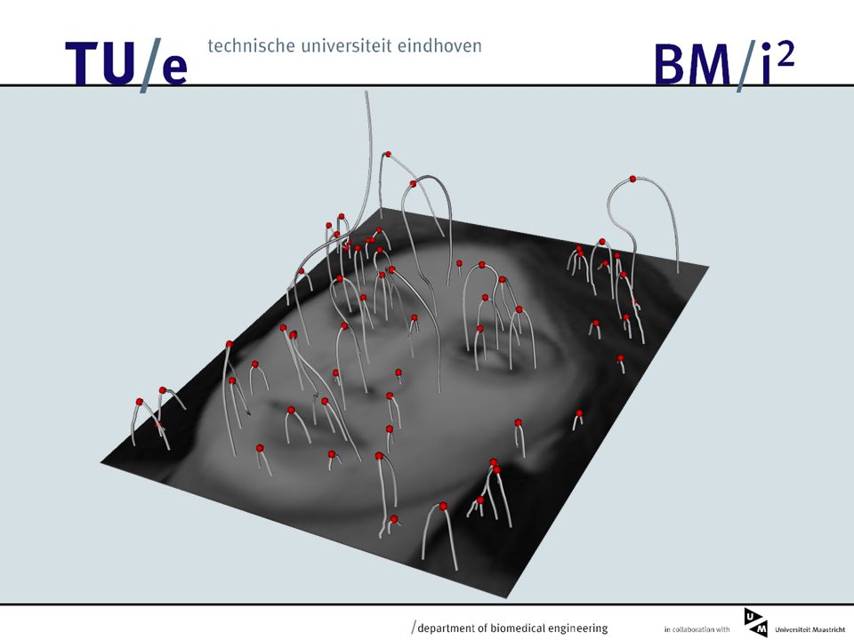
23. Reconstruction It is possible to make a reconstruction of the original image from its top-points. We can generate reconstructed images which give the same (plus more) top- points as the original image. This reconstruction resembles the original image.

24. Original Image Top-Points and Features Reconstruction

25. Metameric Class Original By adjusting boundary and smoothness constraints we can improve the visual performance. For this 300x300 picture 1000 top-points with 6 features were used.

26. This tells us that the top-points indeed contain a lot of information about the image.

27. Localization of Top-Points For points close to top-points it is possible to calculate a vector pointing towards the position of the top-point. x y  Approximated Top- Points Displacement Vectors Real Locations

28. Localization of Top-Points For points close to top-points it is possible to calculate a vector pointing towards the position of the top-point. This enables us to use fast top-point detection algorithms which do not have to be very accurate.

29. Stability of Top-Points The locations of top-points change when noise is added to the image.

31. Stability of Top-Points We can calculate the variance of the displacement of top- points under noise. We need 4 th order derivatives in the top-points for that.

32. Selecting Stable Paths Large instabilities are found in flat areas in the image. Areas with a lot of structure result in more stable top points. In the article we used an adapted version of the TV-norm (Total Variation) to measure the flatness around a top point. We can give top points a weight in the EMD algorithm based on the stability of the point.

33. Calculating the Stability Norm Taylor Expansion (2 nd order) Limiting Procedure Koenderink’s deviation from flatness xcxc x  Integration Area

34. Thresholding on Stability Stable Paths Unstable Paths

35. 123458796 Database Image Retrieval Databas e Query Image

36. Experiments A simple image retrieval task. Using a small version of the Olivetti Faces Database. Consisting of 200 images of 20 different people (10 p.p.)

37. The Deep Structure of an Image Look at all scales simultaneously Scale x y

38. Critical Points, Paths and Top Points Maxima Minimum Saddles  u=0 Critical Points Det(H)=0 Top Points

40. Comparing Top Points of Images CompareEMD

41. Earth Movers Distance (EMD) wiwi f ij c ij AB ujuj [*]Rubner, Tomasi, Guibas, 1998, IEEE Conf. on Computer Vision PilesHoles

42. Calculating the EMD To calculate the earth movers distance we need: –Weights for our top points (e.g. more important points could contain more weight). –A cost function for transporting the weights between point sets (we incorporated a distance function between top points). MMA

43. Measuring Distance in Scale Space Scale Space is not a Euclidean Space. The simple Euclidean Metric no longer holds. Scale x y

44. Eberly’s Distance Measure in Scale Space For an infinitely small step in scale space the following distance function holds: Given this distance function we can find a unique geodesic path connecting two points in scale space. The distance between two points is measured along the this geodesic path connecting these points.  0 relates the importance of scale- to spatial measurements

45. Distance Between Points in Scale Space By parameterizing along the geodesic path the distance function can be derived by solving an ordinary differential equation. This yields the following equation describing the distance between two points in scale space:

46. We now have a distance measure which we can use in our EMD algorithm. We have introduced a tunable parameter  (>0). We now need to give a weight to our points.

47. Results 123456789 a93%78%68%62%58%54%49%45%43% b93%82%90%73%70%68%63%59%56% c95%88%83%76%73%66%62%59%58% d100 % 97%96%95%92%88%86%84%81% a.Using Euclidean Distance b.Using Eberly Distance c.As b. including stability norm d.As c. including 2 nd order derivatives.

48. Distinctive Features To distinguish top-points from each other a set of distinctive features are needed in every top-point. These local features describe the neighborhood of the top-point.

49. Differential Invariants We use the complete set of irreducible 3 rd order differential invariants. These features are rotation and scaling invariant.

50. Matching With the top-points as interest points and the differential invariants as the descriptors we can now start matching them across images.

51. The Task We have a scene and from that scene we want to retrieve the location of the query object.

52. The first step of the matching algorithm is to find the location of our highly invariant interest points, the top-points.

53. The top-points and differential invariants are calculated for the query object and the scene.

54. The location in scale-space (x,y,  ), the gradient angle  and the differential invariant features (D1,D2,D3,D4,D5,D6) are stored for every top-point.

55. Distance between Feature Vectors A sensible distance between feature vectors is essential. We have used Euclidean distance on ‘normalized’ differential invariants. We tried Mahalanobis distance obtained from a training set.

56. Drawbacks of these Methods Euclidean distance is not optimal since the normalization of the features still does not make them Euclidean. The covariance matrix C of the Mahalanobis distance is global and not defined for each feature vector and training is required.

57. Similarity Measure We can calculate the propagation of noise in scale space* This enables us to calculate a covariance matrix  for each feature vector. The dissimilarity (“distance”) measure is expressed as: *Topological and Geometrical Aspects of Image Structure, Johan Blom

58. Improvement Improvement e.g. for 5% noise addition. True Positive Rate False Positive Rate

59. ROC curves

60. We now compare the differential invariant features. compare distance = 0.5distance = 0.2distance = 0.3

61. The vectors with the smallest distance are paired. smallest distance distance = 0.2

62. A set of coordinates is formed from the differences in scale (Log(  o1 )- Log(  s2 )) and in angles (  o1 -  s2 ). (  ,   )

63.   Important Clusters For these clusters we calculate the mean  and  Clustering ( ,  ) If these coordinates are plotted in a scatter plot clusters can be identified. In this scatter plot we find two dense clusters

64. The stability criterion removes much of the scatter

65. After finding  and  for each cluster we transform the (x,y,  ) parameters of the object top-points to match the scene.

66. Rotate and scale according to the cluster means.

67. After this step we can find the translation of the points in scene. By again doing the clustering but now for coordinates (  x,  y).

68. The translations we find correspond to the location of the objects in the scene.

69. In this example we have two clusters of correctly matched points. C1 C2

70. The transformation of each object in the scene matching to the query object is known from the clustering.

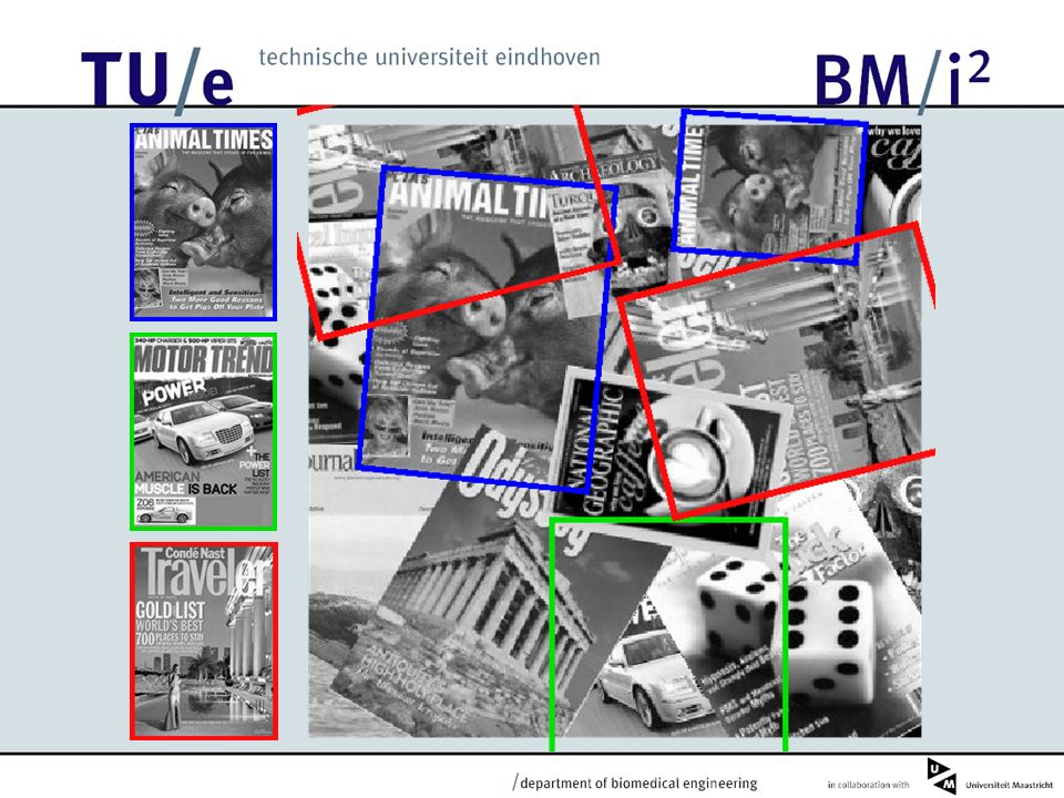
71. We can transform the outline of the query object and project it on the scene image.

72. Object Retrieval Results

74. Invariance to Sampling

76. Conclusion Top-points have proved to be invariant interest points which are useful for matching. The differential invariants have shown to be very distinctive. Experiments show good results.