Download presentation
Presentation is loading. Please wait.

1
Analysis of Thin Wire Antennas Author: Rahul Gladwin. Advisor: Prof. J. Jin Department of Electrical and Computer Engineering, UIUC.

2
Introduction When we design antennas, it is vital to be able to estimate the current distribution on its surface. From the current distribution, we can calculate the input impedance, gain and the far-field pattern for the antenna.

3
Introduction (cont…) Theoretical calculations may be used to analyze antennas with simple geometry, however, as we begin to analyze coupled antennas, the work becomes more tedious. It becomes necessary to numerically model the antenna to determine its current distribution.

4
Introduction (cont…) In this project, I have written a MATLAB program to model the current distribution on thin-wire single and coupled one-dimensional antennas. The algorithm used to evaluate the integrals is based on the Method of Moments and Hallén-Pocklington equations

5
Introduction (cont…) To test my program, I have the modeled current distributions on a single dipole antenna and due to the mutual coupling between closely spaced linear antennas like those in a three-element Yagi-Uda array antenna.
 To test my program, I have the modeled current distributions on a single dipole antenna and due to the mutual coupling between closely spaced linear antennas like those in a three-element Yagi-Uda array antenna.")
6
Theoretical Formulation This purpose of this program is to determine the electric charge density and electric current density that result when an impressed electric field acts on a one dimensional thin wire antenna.

7
Theoretical Formulation (cont…) Until now, we’ve assumed that J is known and we have solved for E. I have now turned this around and solved for J using a known E. Where J is the current density and E is the electric field intensity.

8
Theoretical Formulation (cont…) Obviously, E is not known anywhere, but we do know that E tan = 0 on the surface of the PEC (Perfect Electric Conductor). My further derivations take off from here.

9
Theoretical Formulation (cont…) When studying antennas, we can run into two situations: receiving and transmitting antennas. A successful program should consider both these situations and the differences, if any, should be incorporated in the algorithm. I started by drawing the two scenarios and writing out the respective equations.

10
Transmitting Antennas

11
Receiving Antennas

12
Theoretical Formulation (cont…) The important thing to realize is that whether we’re dealing with either of the two situations, the impressed Electric field induces a current J to flow on and in the wire. J ( r ), in turn produces a scattered field E s. The total electric field produced is E = E i + E s.
, in turn produces a scattered field E s. The total electric field produced is E = E i + E s..")
13
Theoretical Formulation (cont…) For simplicity, I assumed the wires to be perfectly conducting. Thus, the tangential component of the total field must be zero on perfectly conducting wires. This leads to an integral equation that can be solved for J. Once J is known, it can be used to find the required current distribution.

14
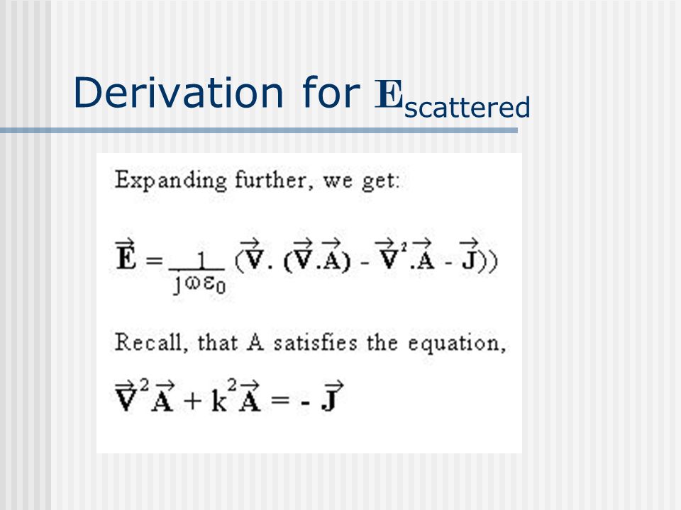
Theoretical Formulation (cont…) Now, all I needed is the expression for E tan on the wire surface that is in terms of the unknown J. The first step is to find an equation relating E to J. It can be derived as follows.

15
Derivation for E scattered

19
The above is the exact solution

20
Simplifying assumptions The wire is a PEC (Perfect Electric Conductor). Current flows only on the surface of the wire. Current only flows on the + axis and is uniformly distributed over the wire surface.

21
Simplifying assumptions (cont…) The wire is thin. I assumed this to enforce that E tan = 0 on PEC wire. Both E z and E phi are tangential components but the thin wire assumptions don’t allow a E phi component. So I only cared about the z-component of E tan.

22
Simplifying assumptions (cont…) From the previous assumptions, I can write the current density within the wire as:
 From the previous assumptions, I can write the current density within the wire as:")
23
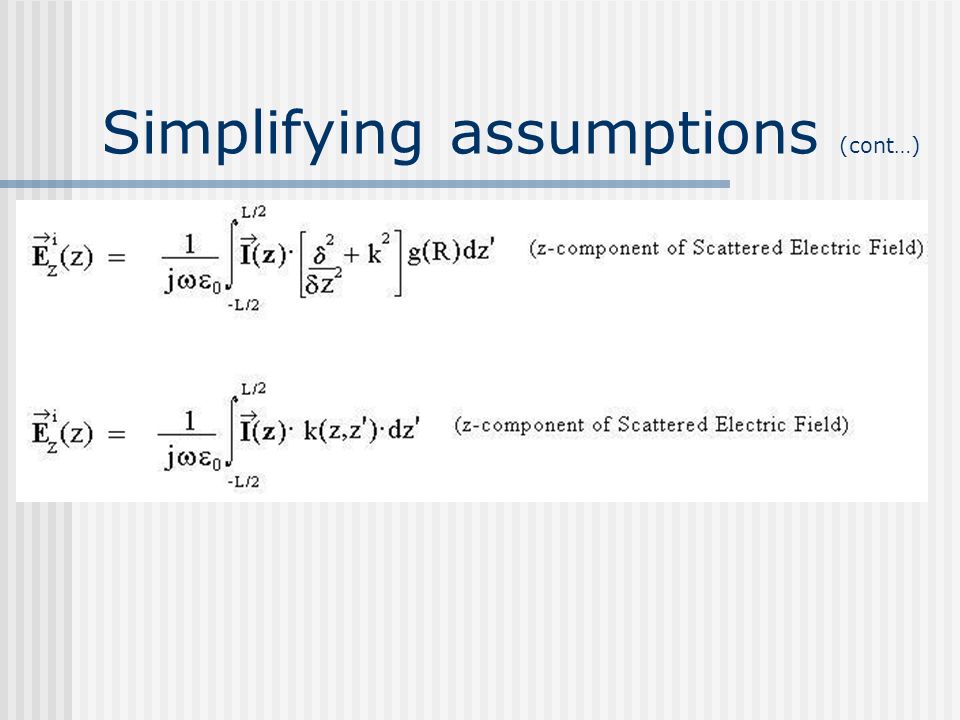
Simplifying assumptions (cont…) After enforcing E tan = 0; by symmetry, E tan = E phi Again, putting down only the z- component of the scattered electric field equation, we get:
 After enforcing E tan = 0; by symmetry, E tan = E phi Again, putting down only the z- component of the scattered electric field equation, we get:")
24
Simplifying assumptions (cont…)
")
25
This is my main equation for evaluating E z. However, there is a problem with the above equation: a singularity exists.

26
Simplifying assumptions (cont…)
")
28
Integral Equation of the First Kind is found: Note that the previous equation can be changed to n equations and n unknowns. That is, the above equation can be solved by discretizing, that is, writing I (z’) as, Integral equation of the first kind (above)
 as, Integral equation of the first kind (above).")
29
Basis function: Triangular

30
Weighting function: Delta The Delta function amounts to forcing E tan =0 only at a discrete set of points. The weighting function is equal to the delta function.

31
Weighting function: Delta In other words, I’m forcing the weighted average of E tan =0 within each interval to be zero. The system becomes: The above is the n th equation

32
Final system of equations Once the above equation is inverted, you can find the current distribution for a whole range of antenna excitations.

33
The Final Equation: Once In is known, we can calculate patterns, gain, etc. of the antenna

34
Analysis of a Straight Dipole An example follows.

35
The Straight Dipole This section provides results from simulations of a 47 cm straight dipole. The straight dipole is analyzed at resonance (300Mhz) in order to validate the model.
 in order to validate the model..")
36
The Straight Dipole (cont…) In order to test my program, I simulated the following 47 cm long dipole because it should exhibit resonance at around 300Mhz.
 In order to test my program, I simulated the following 47 cm long dipole because it should exhibit resonance at around 300Mhz.")
37
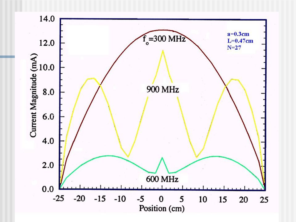
The Straight Dipole (cont…) For analyzing a straight dipole, the program prompts for the number of moments used and the frequency as initial inputs. Based on the derivations, the program then plots the current magnitude as the functions of positions on the dipole.

38
The Straight Dipole (cont…) I used a moment density of 55 moments per wavelength and frequencies of 300Mhz, 600Mhz and 900Mhz. The output follows:

40
Analyzing coupled antennas Numerical Solutions to the Hallén- Pocklington equations for coupled dipoles

41
Theoretical Formulation Here, I discuss their numerical solution. For K antennas in line, on the p th antenna, we have:

42
Theoretical Formulation (cont…) In the above equation, V p (z) is defined to be the sum of the (scaled) vector potentials due to the currents on all antennas:
 In the above equation, V p (z) is defined to be the sum of the (scaled) vector potentials due to the currents on all antennas:")
43
Theoretical Formulation (cont…) The Impedance kernel is:
 The Impedance kernel is:")
44
Theoretical Formulation (cont…) For the P th antenna, the solution for V(p) is of the form:
 For the P th antenna, the solution for V(p) is of the form:")
45
Theoretical Formulation (cont…) Assuming that all the antennas are center driven, we obtain the coupled system of Hallén equations, for p = 1, 2,..., K:
 Assuming that all the antennas are center driven, we obtain the coupled system of Hallén equations, for p = 1, 2,..., K:")
46
Theoretical Formulation (cont…) To solve the previous system of equations, I applied a pulse-function expansion of the form: …and took N = 2M + 1 sampling points on each antenna.
 To solve the previous system of equations, I applied a pulse-function expansion of the form: …and took N = 2M + 1 sampling points on each antenna.")
47
Theoretical Formulation (cont…) On the q th antenna, we have: Therefore, the pulse-function expansion for the q th current must use a square pulse of width delta z q.
 On the q th antenna, we have: Therefore, the pulse-function expansion for the q th current must use a square pulse of width delta z q.")
48
Theoretical Formulation (cont…) Therefore, the current expansion on the qth element should be:
 Therefore, the current expansion on the qth element should be:")
49
Theoretical Formulation (cont…) I used the previous equation and sampled along the p th antenna …and obtained the discretized Hallén system as:
 I used the previous equation and sampled along the p th antenna …and obtained the discretized Hallén system as:")
50
Theoretical Formulation (cont…) The previous equation can be written in a more compact form since p=1,2,3…K. The new form is:

51
Theoretical Formulation (cont…) Now, n-dimensional vectors can me defined:
 Now, n-dimensional vectors can me defined:")
52
Theoretical Formulation (cont…) This system provides k coupled matrix equations by which we can determined the k sampled currents on the antennas. For example, if k=3, we have:

53
Theoretical Formulation (cont…) This matrix can also be written in the form:
 This matrix can also be written in the form:")
54
Theoretical Formulation (cont…) The solution to this equation is of the form: I have written a MATLAB script that solves the above equation for currents on coupled antennas.
 The solution to this equation is of the form: I have written a MATLAB script that solves the above equation for currents on coupled antennas.")
55
Analysis of a Three element Yagi-Uda array An Example follows

56
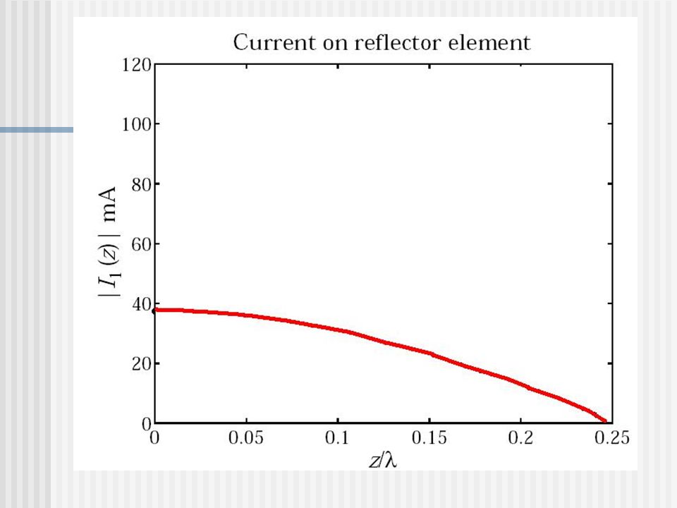
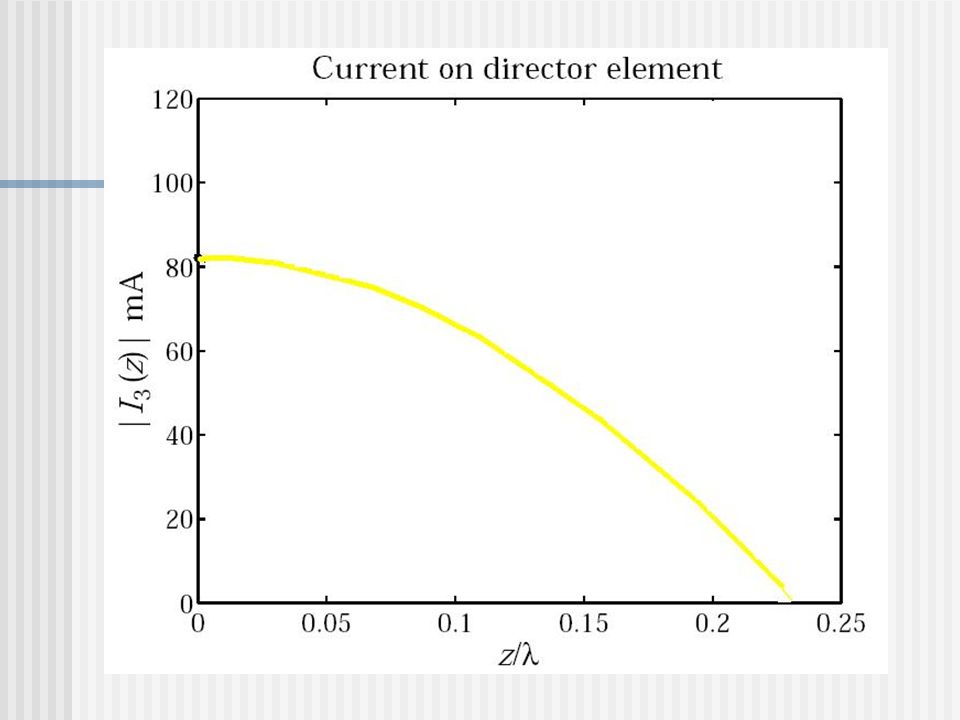
Yagi-Uda array The three-element Yagi I simulated consisted of one reflector, one driven element and one director. The corresponding antenna lengths, radii and locations on the x-axis (with the driven element at origin) were in units of ‘lambda’ (wavelengths - meter)
 were in units of ‘lambda’ (wavelengths - meter).")
57
Yagi-Uda array (cont…) My program prompts the values of ‘L’, ‘a’ and ‘d’ as inputs. L=antenna length, a=radius and d=distance along the horizontal axis. Here is the data I used:

61
Reference 1.Harrington, Roger F., Field Computation by Moment Methods. New York: IEEE Press, 1993. 2.Micheilssen, Eric. ECE 354 Lecture Notes on Antennas. The University of Illinois at Urbana-Champaign, 2003. 3.Janaswamy, Ramakrishna. Radiowave Propagation and Smart Antennas for wireless communications, Kluwe Academic Publishers, Boston, 1999. 4.IEEE Antennas and Propagation Magazine, Vol 44, No. 4, August 2002. 5. Pozar, David. Microstrip Antennas : The Analysis and Design of Microstrip Antennas and Arrays, Wiley-IEEE Press, July 1995.

62
Special Thanks To Prof. J. Jin and his research group

Similar presentations


![Time Domain Analysis of the Multiple Wires Above a Dielectric Half-Space Poljak [1], E.K.Miller [2], C. Y. Tham [3], S. Antonijevic [1], V. Doric [1] [1]](/15/4661669/big_thumb.jpg "Time Domain Analysis of the Multiple Wires Above a Dielectric Half-Space Poljak [1], E.K.Miller [2], C. Y. Tham [3], S. Antonijevic [1], V. Doric [1] [1]>")


