1. Marlon Dumas marlon.dumas ät ut . ee
MTAT Business Process Management (BPM) Lecture 6 Quantitative Process Analysis (Queuing & Simulation)
Marlon Dumas
marlon.dumas ät ut . ee

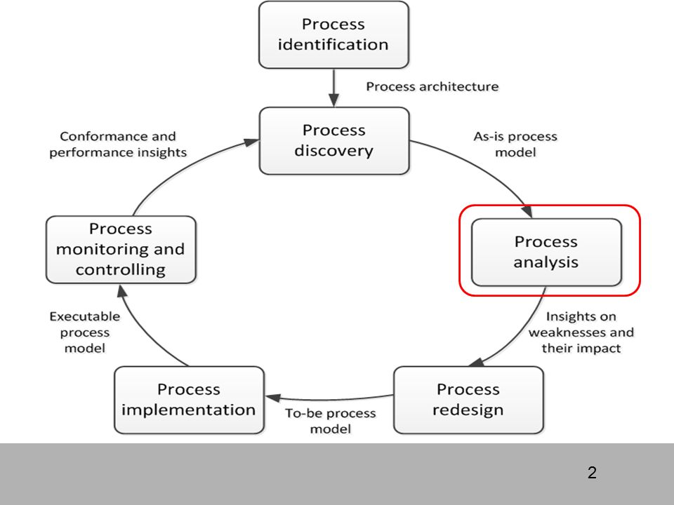
3. Process Analysis Techniques
Quantitative Analysis
Quantitative Flow Analysis
Queuing Theory
Process Simulation
Qualitative analysis
Value-Added Analysis
Root-Cause Analysis
Pareto Analysis
Issue Register

4. Why flow analysis is not enough?
Flow analysis does not consider waiting times due to resource contention
Queuing analysis and simulation address these limitations and have a broader applicability

5. Why is Queuing Analysis Important?
Capacity problems are very common in industry and one of the main drivers of process redesign
Need to balance the cost of increased capacity against the gains of increased productivity and service
Queuing and waiting time analysis is particularly important in service systems
Large costs of waiting and/or lost sales due to waiting
Prototype Example – ER at a Hospital
Patients arrive by ambulance or by their own accord
One doctor is always on duty
More patients seeks help  longer waiting times
Question: Should another MD position be instated?
© Laguna & Marklund

6. Delay is Caused by Job Interference
Deterministic traffic
Variable but spaced apart traffic
Queuing occurs every time user demand exceeds server capacity.
Delays are due to several reasons. Let’s examine some of them…
If arrivals are regular or sufficiently spaced apart, no queuing delay occurs
© Dimitri P. Bertsekas

7. Burstiness Causes Interference
Queuing results from variability in service times and/or interarrival intervals
What does “bursty traffic” mean?
© Dimitri P. Bertsekas

8. Job Size Variation Causes Interference
Arrivals are deterministic (e.g. the intervals between 2 consecutive arrivals are always the same), however some jobs are longer than others
Deterministic arrivals, variable job sizes
© Dimitri P. Bertsekas

9. High Utilization Exacerbates Interference
The queuing probability increases as the load increases
Utilization close to 100% is unsustainable  too long queuing times
Delay probability is higher under heavy loading conditions than when the traffic is light
© Dimitri P. Bertsekas

10. The Poisson Process
Common arrival assumption in many queuing and simulation models
The times between arrivals are independent, identically distributed and exponential
P (arrival < t) = 1 – e-λt
Key property: The fact that a certain event has not happened tells us nothing about how long it will take before it happens
e.g., P(X > 40 | X >= 30) = P (X > 10)
A useful queuing model represents a real-life system with sufficient accuracy and is analytically tractable. A queuing model based on the Poisson process often meets these two requirements. A Poisson process models random events (such as a customer arrival, a request for action from a web server, or the completion of the actions requested of a web server) as emanating from a memoryless process. That is, the length of the time interval from the current time to the occurrence of the next event does not depend upon the time of occurrence of the last event
Independent increments: the numbers of occurrences counted in disjoint intervals are independent from each other
Stationary increments: the probability distribution of the number of occurrences counted in any time interval only depends on the length of the interval
Closed under Addiction and Subtraction
© Laguna & Marklund

11. Negative Exponential Distribution

12. Queuing theory: basic concepts
service
waiting
arrivals l c m
Basic characteristics:
l (mean arrival rate) = average number of arrivals per time unit
m (mean service rate) = average numberof jobs that can be handled by one server per time unit:
c = number of servers
© Wil van der Aalst

13. Queuing theory concepts (cont.)l c m
Wq,Lq
W,L
Given l , m and c, we can calculate :
occupation rate: r
Wq = average time in queue
W = average system in system (i.e. cycle time)
Lq = average number in queue (i.e. length of queue)
L = average number in system average (i.e. Work-in-Progress)
© Wil van der Aalst

14. M/M/1 queue l 1 m Assumptions:
time between arrivals and service time follow a negative exponential distribution
1 server (c = 1)
FIFO
L=/(1- )
Lq= 2/(1- ) = L-
W=L/=1/(- )
Wq=Lq/=  /( (- ))
© Laguna & Marklund

15. M/M/c queue
Now there are c servers in parallel, so the expected capacity per time unit is then c*
Little’s Formula  Wq=Lq/
W=Wq+(1/)
Little’s Formula  L=W
© Laguna & Marklund

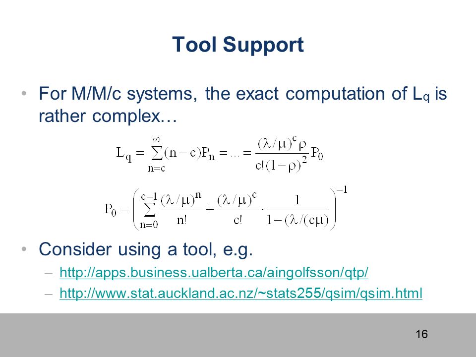
16. Tool Support
For M/M/c systems, the exact computation of Lq is rather complex…
Consider using a tool, e.g.

17. Example – ER at County Hospital
Situation
Patients arrive according to a Poisson process with intensity  ( the time between arrivals is exp() distributed.
The service time (the doctor’s examination and treatment time of a patient) follows an exponential distribution with mean 1/ (=exp() distributed)
The ER can be modeled as an M/M/c system where c=the number of doctors
Data gathering
 = 2 patients per hour
 = 3 patients per hour
Question
Should the capacity be increased from 1 to 2 doctors?
© Laguna & Marklund

18. Queuing Analysis – Hospital Scenario
Interpretation
To be in the queue = to be in the waiting room
To be in the system = to be in the ER (waiting or under treatment)
Is it warranted to hire a second doctor ?
Characteristic
One doctor (c=1)
Two Doctors (c=2) 
2/3
1/3 Lq
4/3 patients
1/12 patients L
2 patients
3/4 patients Wq
2/3 h = 40 minutes
1/24 h = 2.5 minutes W
1 h
3/8 h = 22.5 minutes
© Laguna & Marklund

19. Process Simulation Drawbacks of queuing theory:
Generally not applicable when system includes parallel activities
Requires case-by-case mathematical analysis
Assumes “steady-state” (valid only for “long-term” analysis)
Process simulation is more versatile (also more popular)
Process simulation = run a large number of process instances, gather data (cost, duration, resource usage) and calculate statistics from the output

20. Process Simulation Steps in evaluating a process with simulation
Model the process (e.g. BPMN)
Enhance the process model with simulation info  simulation model
Based on assumptions or better based on data (logs)
Run the simulation
Analyze the simulation outputs
Process duration and cost stats and histograms
Waiting times (per activity)
Resource utilization (per resource)
Repeat for alternative scenarios

21. Elements of a simulation model
The process model including:
Events, activities, control-flow relations (flows, gateways)
Resource classes (i.e. lanes)
Resource assignment
Mapping from activities to resource classes
Processing times
Per activity or per activity-resource pair
Costs
Per activity and/or per activity-resource pair
Arrival rate of process instances
Conditional branching probabilities (XOR gateways)

22. Simulation Example – BPMN model

23. Resource Pools (Roles)
Two options to define resource pools
Define individual resources of type clerk
Or assign a number of “anonymous” resources all with the same cost
E.g.
3 anonymous clerks with cost of € 10 per hour, 8 hours per day
2 individually named clerks
Jim: € 12.4 per hour
Mike: € 14.8 per hour
1 manager John at € 20 per hour, 8 hours per day

24. Resource pools and execution times
Task
Role
Execution Time
Normal distribution: mean and std deviation
Receive application
system
Check completeness
Clerk
30 mins
10 mins
Perform checks
2 hours
1 hour
Request info
1 min
Receive info (Event)
48 hours
24 hours
Make decision
Manager
Notify rejection
Time out (Time)
72 hours
Receive review request (Event)
12 hours
Notify acceptance
Deliver Credit card
Alternative: assign execution times to the tasks only (like in cycle time analysis)

25. Reminder: Normal Distribution

26. Arrival rate and branching probabilities
10 applications per hour (one at a time)
Poisson arrival process (negative exponential)
0.3
0.5
0.7
0.8
0.5
0.2
Alternative: instead of branching probabilities one can assign “conditional expressions” to the branches based on input data

27. Simulation output: KPIs

28. Simulation output: detailed logs
Process Instance
# Activities
Start
End
Cycle Time
Cycle Time (s)
Total Time 6 5
4/06/ :00
4/06/ :26
03:26:44 7
4/06/ :00
5/06/2007 9:30
19:30:38 11
4/06/ :00
5/06/ :14
18:14:56 13
4/06/ :00
5/06/ :14
17:14:56 16
4/06/ :00
5/06/ :06
16:06:29 22
5/06/2007 5:00
6/06/ :01
29:01:39 27 8
5/06/ :00
6/06/ :33
26:33:21
Process Instance
Activity ID
Activity Name
Activity Type
Resource
Start
End 6
aed54717-f044-4da1-b543-82a660809ecb
Check for completeness
Task
Manager
4/06/ :00
4/06/ :53
a270f5c6-7e16-42c1-bfc4-dd10ce8dc835
Perform checks
Clerk
4/06/ :25
77511d7c-1eda-40ea-ac7d-886fa03de15b
Make decision
4/06/ :26
099a64eb e6-e7de36d348c2
Notify acceptance
IntermediateEvent
(none)
0a72cf f31-8c7e-6d093429ab04
Deliver card
System
4/06/ :26 7
4/06/ :00
4/06/ :31
5/06/2007 8:30

29. Tools for Process Simulation
Not exhaustive, listed in no specific order:
ITP Commerce Process Modeler for Visio
Bizagi Process Modeler
Progress Savvion Process Modeler
ARIS
Oracle BPA
ProSim
BIMP

30. Simple Online Simulator
BIMP:
Accepts standard BPMN 2.0 as input
Link from Signavio Academic Edition to BIMP
Open a model in Signavio and push it to BIMP using the flask icon

31. BIMP Demo