Download presentation
Presentation is loading. Please wait.

1
What is Millimetre-Wave Astronomy and why is it different? Michael Burton University of New South Wales

2
Some Millimetre Basics MM: 1–~12mm, Sub-MM: 0.3–1mm CMBR (T = 2.7K = 1mm) Molecular rotational lines –Polar molecules (have dipole moment) eg CO (E 1 = 5K), HCN, CS, HCO + Cold thermal continuum (dust) –Thermal processes: F ~ B ~ 2kT 2 /c 2. x Problem: Atmosphere (O 2, H 2 O)……
…….")
3
The Millimetre Advantage Thermal Processes B 0.5-2 2 Decay Rates (linear molecules) 3 Doppler Widths 0.5 [?] Level Population (T>>T J ; g J J) Number of Photons -1 Energy Spatial Resolution -1
![The Millimetre Advantage Thermal Processes B Decay Rates (linear molecules) 3 Doppler Widths 0.5 [ ] Level Population (T>>T J ; g J J) Number of Photons -1 Energy Spatial Resolution -1](http://images.slideplayer.com/24/7431863/slides/slide_3.jpg "The Millimetre Advantage Thermal Processes B Decay Rates (linear molecules) 3 Doppler Widths 0.5 [ ] Level Population (T>>T J ; g J J) Number of Photons -1 Energy Spatial Resolution -1")
4
Transparancies Electromagnetic Spectrum MM transmission for 4mm H 2 O MM transmission for 11mm H 2 O Some bright MM-lines

5
Brightness Temperature

6
Atmospheric Transmission

7
The 3mm Millimetre Spectrum

8
Physical Parameters you can derive! Temperature: T ex, T Brightness Density: n H2 (~n crit range of densities present!) Column Density: N (when optically thin) Optical Depth: (use isotope ratios) Mass (with scale length) Abundances: different species Velocities: line widths, centres, shapes Infall, outflow, mass transfer rates Constrain the properties of your source!!
 Column Density: N (when optically thin) Optical Depth: (use isotope ratios) Mass (with scale length) Abundances: different species Velocities: line widths, centres, shapes Infall, outflow, mass transfer rates Constrain the properties of your source!!.")
9
16272-4837 SEST molecular line survey –Gradient: T rot = 27 ± 4 K –Intercept: N(H 2 ) = 1 x 10 24 cm -2 ( comes in as well) – Size + Column: n(H 2 ) = 6 x 10 5 cm -3 – With Volume: Mass = 6 x 10 3 M Garay et al, 2002
 = 1 x cm -2 ( comes in as well) – Size + Column: n(H 2 ) = 6 x 10 5 cm -3 – With Volume: Mass = 6 x 10 3 M Garay et al, 2002")
10
16272-4837: SEST kinematical studies – Evidence for infall (profile of optically thick lines) - Modelling: V infall ~ 0.5 km s -1 - Speed + Density + Size: dM infall /dt ~10 -2 M yr -1 – Evidence for outflow from wings - Extent: V outflow = 15 km s -1 Brooks et al, 2002 Optically Thick Optically Thin Wide Wings
 - Modelling: V infall ~ 0.5 km s -1 - Speed + Density + Size: dM infall /dt ~10 -2 M yr -1 – Evidence for outflow from wings - Extent: V outflow = 15 km s -1 Brooks et al, 2002 Optically Thick Optically Thin Wide Wings")
12
Mopra: Current Capabilities 22-m Telescope for > ~3mm 85–115 GHz SIS receiver (2.6 – 3.5 mm) 35” beam @ 100 GHz T sys ~ 150K(@85GHz) – 300K (@115GHz) Beam Efficiency: – mb (86 GHz) = 0.49, mb (115 GHz) = 0.42 – xb (86 GHz) = 0.65, xb (115 GHz) = 0.55 Bandwidth 64, 128 or 256 MHz (200 - 800 km/s) 1024 Channels (0.2 - 0.8 km/s per channel) 2 Polarizations –1 frequency or 1 polarization + SiO 86 GHz Must Nod – No chopping OTF Mapping
 GHz T sys ~ – 300K Beam Efficiency: – mb (86 GHz) = 0.49, mb (115 GHz) = 0.42 – xb (86 GHz) = 0.65, xb (115 GHz) = 0.55 Bandwidth 64, 128 or 256 MHz ( km/s) 1024 Channels ( km/s per channel) 2 Polarizations –1 frequency or 1 polarization + SiO 86 GHz Must Nod – No chopping OTF Mapping")
13
Methanol Maser-selected Hot Molecular Core Survey CH 3 CN CH 3 OH HCO + H 13 CO + N 2 H + HCN HNC 7 lines; 86 Sources Purcell

14
‘On the Fly’ Mapping with Mopra: The Horsehead Nebula Optical 12 CO 13 CO 6 arcmin Tony Wong

15
0.17 km/s channel spacing

16
OTF Mapping Specifications For a 300” x 300” map: –~1400 spectra (31 x 46) –~35” resolution –0.17 km/s resolution –120 km/s bandwidth –Dual polarization – ~ 0.3K per channel, per beam –~70 minutes / grid –Upto 7 grids / transit –Processed with LIVEDATA + GRIDZILLA packages
 –~35 resolution –0.17 km/s resolution –120 km/s bandwidth –Dual polarization – ~ 0.3K per channel, per beam –~70 minutes / grid –Upto 7 grids / transit –Processed with LIVEDATA + GRIDZILLA packages")
17
The DQS in 13 CO: Mopra OTF Mapping

18
How many photons have we lost (or gained)? 00 0 sec(z) z Signal on-source: T rec T sou T atm
 00 0 sec(z) z Signal on-source: T rec T sou T atm")
19
Sky (Reference, Off) Source (On) Difference
 Source (On) Difference")
20
Some Radiative Transfer Radiative TransferdI /ds = - I + Kirchoff (LTE) / = B (T) Radiative TransferdI /d = I + B (T) SolutionI (s)= I (0)e - (s) + B (T)(1 - e - (s) ) Source Atmosphere
 / = B (T) Radiative TransferdI /d = I + B (T) SolutionI (s)= I (0)e - (s) + B (T)(1 - e - (s) ) Source Atmosphere")
21
Obtaining Data: Signal from Source and Reference T Sig = C{T R +T A (1-e - 0 secz )+T S e - 0 secz } T Ref = C{T R +T A (1-e - 0 secz )} [T Sig -T Ref ]/[T Ref ] = T S e - 0 secz / {T R +T A (1-e - 0 secz )} Show Plots of Opacity + Brightness Temperature T BB = C{T R +T A } [T Sig -T Ref ]/[T BB - T Ref ] = T S /T A
![Obtaining Data: Signal from Source and Reference T Sig = C{T R +T A (1-e - 0 secz )+T S e - 0 secz } T Ref = C{T R +T A (1-e - 0 secz )} [T Sig -T Ref ]/[T Ref ] = T S e - 0 secz / {T R +T A (1-e - 0 secz )} Show Plots of Opacity + Brightness Temperature T BB = C{T R +T A } [T Sig -T Ref ]/[T BB - T Ref ] = T S /T A](http://images.slideplayer.com/24/7431863/slides/slide_21.jpg "Obtaining Data: Signal from Source and Reference T Sig = C{T R +T A (1-e - 0 secz )+T S e - 0 secz } T Ref = C{T R +T A (1-e - 0 secz )} [T Sig -T Ref ]/[T Ref ] = T S e - 0 secz / {T R +T A (1-e - 0 secz )} Show Plots of Opacity + Brightness Temperature T BB = C{T R +T A } [T Sig -T Ref ]/[T BB - T Ref ] = T S /T A")
22
Calibrating Data: Gated Total Power GTP Ref = C’ T Ref GTP Paddle = C’{T A + T R } [GTP Paddle - GTP Ref ] / GTP Ref = T A e - 0 secz / {T R +T A (1-e - 0 secz )} GTP Hot - GTP Cold = C’{T Hot - T Cold } Atmosphere Liquid Nitrogen
![Calibrating Data: Gated Total Power GTP Ref = C’ T Ref GTP Paddle = C’{T A + T R } [GTP Paddle - GTP Ref ] / GTP Ref = T A e - 0 secz / {T R +T A (1-e - 0 secz )} GTP Hot - GTP Cold = C’{T Hot - T Cold } Atmosphere Liquid Nitrogen](http://images.slideplayer.com/24/7431863/slides/slide_22.jpg "Calibrating Data: Gated Total Power GTP Ref = C’ T Ref GTP Paddle = C’{T A + T R } [GTP Paddle - GTP Ref ] / GTP Ref = T A e - 0 secz / {T R +T A (1-e - 0 secz )} GTP Hot - GTP Cold = C’{T Hot - T Cold } Atmosphere Liquid Nitrogen")
23
Calibrating Data: {[T Sig -T Ref ]/[T Ref ]} / {[GTP Paddle - GTP Ref ] / GTP Ref } = T Source / T Atmosphere Actually T Source = T’ Source / Efficiency –Usually written as T MB = T A * / (note the different notation)
![Calibrating Data: {[T Sig -T Ref ]/[T Ref ]} / {[GTP Paddle - GTP Ref ] / GTP Ref } = T Source / T Atmosphere Actually T Source = T’ Source / Efficiency –Usually written as T MB = T A * / (note the different notation)](http://images.slideplayer.com/24/7431863/slides/slide_23.jpg "Calibrating Data: {[T Sig -T Ref ]/[T Ref ]} / {[GTP Paddle - GTP Ref ] / GTP Ref } = T Source / T Atmosphere Actually T Source = T’ Source / Efficiency –Usually written as T MB = T A * / (note the different notation)")
24
Mopra Upgrades 8 GHz Digital Filter Bank –Zoom modes –4(?) lines simultaneously MMIC receiver –Easier tuning –Higher T sys –May loose 115 GHz end? 7 mm receiver –New ATNF project? Focal Plane Array??? Ultra-wide band correlator??? –Needs source of funds……

25
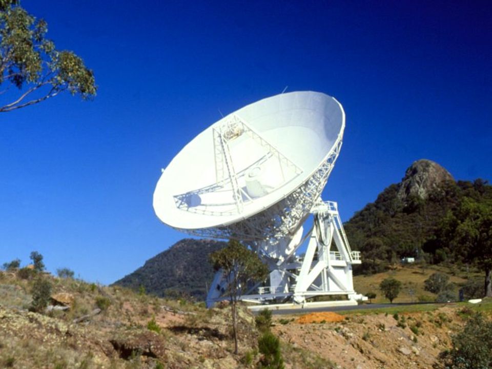
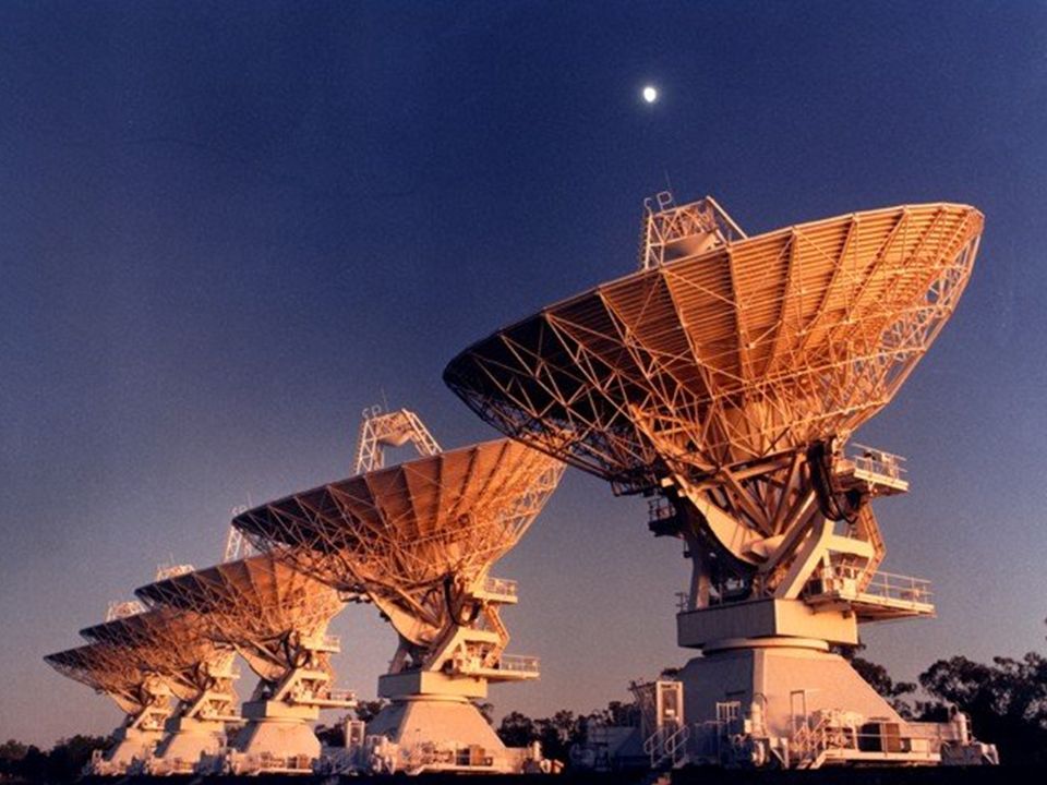
Australia’s MM–Wave Radio Telescopes 3 mm 12 mm

27
Australia Telescope Compact Array National Facility –Built for 1–10 GHz operation MM-upgrades –3 mm (85-~105 (115) GHz) 5 x 22m antennas EW-array + NS-spur –Currently 84.9-87.3+88.5-91.3 GHz –12 mm (22-25 GHz) 6 x 22m antennas 2 GHz bandwidth upgrade 7 mm (45 GHz) upgrade planned –6 antennas FPAs??? –With ultra-wide-band correlators??

28
Water Vapour and Phase Fluctuations

29
Millimetre Interferometry Poses special challenges: Significant atmospheric opacity, mostly due to H 2 O Fluctuations in H 2 O produce phase shifts These increase with both baseline and frequency Instrumental requirements (e.g. surface, pointing, baseline accuracy) are more severe Need more bandwidth to cover same velocity range (1 MHz (mm) km/s) R Sault Desai 1998 Brightness Temperature H 2 O Turbulence Seeing
 are more severe Need more bandwidth to cover same velocity range (1 MHz (mm) km/s) R Sault Desai 1998 Brightness Temperature H 2 O Turbulence Seeing.")
30
ALMA Atacama Large Millimetre Array

31
Antarctica??

Similar presentations

 Molecular Line Surveys of Dark Clouds Discovery of CH 3 O.>")

, ν, Ω S Unknowns: V, T K, N X, M H 2, n H 2 –V velocity field –T K kinetic.>")
 Alan Roy (MPIfR), Christian Henkel (MPIfR)>")


 demonstration survey of the Galactic plane G. Fuller, N. Peretto, L. Quinn (University of Manchester UK), J. Green (ATNF ) All dust continuum.>")


 Todd Hunter (NRAO/North American ALMA Science Center) Collaborators: Crystal Brogan (NRAO) Ken.>")


