1. Change Point Analysis in BioSense 2.0  To access the slides for today’s presentation, go to: https://sites.google.com/site/biosenseredesign/training/tra ining-library (the document name is “CPA_Webinar.pptx”) https://sites.google.com/site/biosenseredesign/training/tra ining-library  Questions may be submitted via the chat feature. Please try to hold questions until the Q&A portion of the webinar. Any questions we cannot answer on today’s webinar will be answered and posted to the Collaboration Site. Technical questions related to webinar difficulties may be submitted via the chat feature at any time.

2. Change Point Analysis in BioSense 2.0 David Buckeridge MD PhD 1 and Nabarun Dasgupta PhD 2 1 Associate Professor, Epidemiology and Biostatistics, McGill University, Canada Research Chair In Public Health Informatics 2 BioSense Redesign Team

3. Introduction to the Change Point Algorithm  One of two aberration detection algorithms currently implemented in BioSense 2.0  The change point algorithm was developed by Taylor  The general idea is to iteratively  Apply cumulative sums to the residuals of a time series  Use resampling of the original series to estimate significance  An application of the change point algorithm to biosurveillance is described by Kass-Hout et al. Taylor, W. Change-Point Analysis: A Powerful New Tool For Detecting Changes. 2010; Available from: http://www.variation.com/anonftp/pub/changepoint.pdf. http://www.variation.com/anonftp/pub/changepoint.pdf Kass-Hout TA, Xu Z, McMurray P, Park S, Buckeridge DL, Brownstein JS, Finelli L, Groseclose SL. Application of change point analysis to daily influenza-like illness emergency department visits. J Am Med Inform Assoc. 2012 Nov-Dec;19(6):1075-81. http://jamia.bmj.com/cgi/content/full/amiajnl-2011-000793

4. Understanding the Change Point Algorithm  Objective: Find the date(s) in a time series where the mean value of the series ‘shifts’ significantly  Algorithm 1.Calculate cumulative sum of the residuals for the time series 2.Find change point — absolute maximum of the cumulative sum 3.Assess significance of change point through resampling 4.Split time series in two on either side of change point and repeat steps 1-3 for each subsection of the time series 5.Report statistically significant change points

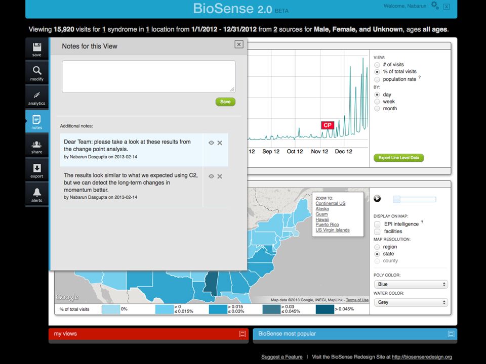
5. An Example Time Series from BioSense 2.0 ILI visits to all DOD and VA facilities between 2012-01-01 and 2012-12-31

6. 1. Cumulative Sum of the Residuals for a Time Series The mean of the series is 0.0419

7. 1. Cumulative Sum of the Residuals for a Time Series DateX(t)ResidualCusum 0 2012-01-010.05520.0132 2012-01-020.08180.03990.0531 2012-01-030.0105-0.03140.0218 2012-01-040.0091-0.0328-0.0110 …………

8. 2. Absolute Maximum of the Cumulative Sum The absolute maximum of the cumulative sum of the residuals is -5.79.

9. 2. Maximum of the Cumulative Sum = Change Point The date at the absolute maximum, or the change point, is 2012-11-10.

10. 3. Assess Significance through Resampling The difference between the maximum and minimum of the cumulative sum of the residuals is used as a measure of the change point.

11. 3. Assess Significance through Resampling A. Shuffle the observed values in the original series so that they are in a random order. B. Measure and record the difference between the maximum and minimum of the cumulative sum of the residuals.

12. 3. Assess Significance through Resampling Repeat...

13. 3. Assess Significance through Resampling Repeat...

14. 3. Assess Significance through Resampling The observed difference is greater than the differences calculated from cumulative sums of 999 permutations of the time series. So, the observed break point is likely to be observed by chance fewer than 1 in 1000 times, or p < 0.001.

15. 3. Assess Significance through Resampling 2012-11-10 ‘Up’ p < 0.001 2012-11-10 ‘Up’ p < 0.001

16. 4. Split Time Series in Two and Repeat on Sub-Series First break point

17. 4. Split Time Series in Two and Repeat on Sub-Series First break point Sub-series A Sub-series B

18. 4. Split Time Series in Two and Repeat on Sub-Series First break point Sub-series A Break point in A Sub-series B Break point in B

19. 5. Report Statistically Significant Change Points 2012-02-18 ‘Up’ p < 0.025 2012-02-18 ‘Up’ p < 0.025 2012-11-10 ‘Up’ p < 0.001 2012-11-10 ‘Up’ p < 0.001 2012-04-09 ‘Down’ p < 0.001 2012-04-09 ‘Down’ p < 0.001

20. Applying the Change Point Algorithm (CPA)  The CPA detects shifts in the mean and indicates the direction of the shift.  Algorithm is straightforward and results are easy to understand.  CPA can be used alone, but probably more informative when used with aberration detection method, such as C2.  Further practical and theoretical results will help to define the role of CPA in surveillance analysis.

34. Upcoming BioSense 2.0 Webinars  A webinar will be scheduled for March; the topic is to be determined.  For more information, please visit our Collaboration Web Site www.biosense2.orgwww.biosense2.org  If you have any suggestions for future webinars, please contact us at info@biosen.seinfo@biosen.se