Download presentation
Presentation is loading. Please wait.

1
Object Recognizing

2
Recognition -- topics Features Classifiers Example ‘winning’ system

3
Object Classes

4
Individual Recognition

5
Object parts Automatic, or query-driven Headlight Window Door knob Back wheel Mirror Front wheel Headlight Window Bumper

6
ClassNon-class

7
Variability of Airplanes Detected

8
Class Non-class

9
Features and Classifiers Same features with different classifiers Same classifier with different features

10
Generic Features: The same for all classes Simple (wavelets)Complex (Geons)
Complex (Geons)")
11
Class-specific Features: Common Building Blocks

12
Optimal Class Components? Large features are too rare Small features are found everywhere Find features that carry the highest amount of information

13
Entropy Entropy: x =01H p =0.50.5? 0.10.90.47 0.010.990.08

14
Mutual information H(C) when F=1H(C) when F=0 I(C;F) = H(C) – H(C/F) F=1 F=0 H(C)
 when F=1H(C) when F=0 I(C;F) = H(C) – H(C/F) F=1 F=0 H(C)")
15
Mutual Information I(C,F) Class:11010100 Feature:10011100 I(F,C) = H(C) – H(C|F)
 Class: Feature: I(F,C) = H(C) – H(C|F)")
16
Optimal classification features Theoretically: maximizing delivered information minimizes classification error In practice: informative object components can be identified in training images

17
Selecting Fragments

18
Horse-class features Car-class features Pictorial features Learned from examples

19
Star model Detected fragments ‘vote’ for the center location Find location with maximal vote In variations, a popular state-of-the art scheme

20
Bag of words

21
Bag of visual words A large collection of image patches –

23
Generate a dictionary using K-means clustering

25
Recognition by Bag of Words (BoD): Each class has its words historgram – – – Limited or no Geometry Simple and popular, no longer state-of-the art.
: Each class has its words historgram – – – Limited or no Geometry Simple and popular, no longer state-of-the art.")
26
HoG Descriptor Dallal, N & Triggs, B. Histograms of Oriented Gradients for Human Detection

27
Shape context

28
Recognition Class II: SVM Example Classifiers

29
SVM – linear separation in feature space

30
Separating line:w ∙ x + b = 0 Far line:w ∙ x + b = +1 Their distance:w ∙ ∆x = +1 Separation:|∆x| = 1/|w| Margin:2/|w| 0 +1 The Margin

31
Max Margin Classification (Equivalently, usually used How to solve such constraint optimization? The examples are vectors x i The labels y i are +1 for class, -1 for non-class

32
Solving the SVM problem Duality Final form Efficient solution Extensions

33
Using Lagrange multipliers: Using Lagrange multipliers: Minimize L P = With α i > 0 the Lagrange multipliers

34
Minimizing the Lagrangian Minimize L p : Set all derivatives to 0: Also for the derivative w.r.t. α i Dual formulation: Maximize the Lagrangian w.r.t. the α i and the above two conditions.

35
Solved in ‘dual’ formulation Maximize w.r.t α i : With the conditions:

36
Dual formulation Mathematically equivalent formulation: Can maximize the Lagrangian with respect to the α i After manipulations – concise matrix form:

37
Summary points Linear separation with the largest margin, f(x) = w∙x + b Dual formulation Natural extension to non-separable classes Extension through kernels, f(x) = ∑α i y i K(x i x) + b
 = w∙x + b Dual formulation Natural extension to non-separable classes Extension through kernels, f(x) = ∑α i y i K(x i x) + b")
38
Felzenszwalb Felzenszwalb, McAllester, Ramanan CVPR 2008. A Discriminatively Trained, Multiscale, Deformable Part Model Many implementation details, will describe the main points.

39
Using patches with HoG descriptors and classification by SVM Person model HoG orientations with w > 0

40
Object model using HoG A bicycle and its ‘root filter’ The root filter is a patch of HoG descriptor Image is partitioned into 8x8 pixel cells In each block we compute a histogram of gradient orientations

41
The filter is searched on a pyramid of HoG descriptors, to deal with unknown scale Dealing with scale: multi-scale analysis

42
A part Pi = (Fi, vi, si, ai, bi). Fi is filter for the i-th part, vi is the center for a box of possible positions for part i relative to the root position, si the size of this box ai and bi are two-dimensional vectors specifying coefficients of a quadratic function measuring a score for each possible placement of the i-th part. That is, a i and b i are two numbers each, and the penalty for deviation ∆x, ∆y from the expected location is a 1 ∆ x + a 2 ∆y + b 1 ∆x 2 + b 2 ∆y 2 Adding Parts

43
Bicycle model: root, parts, spatial map Person model

45
The full score of a potential match is: ∑ F i ∙ H i + ∑ a i1 x i + a i2 y i + b i1 x i 2 + b i2 y i 2 F i ∙ H i is the appearance part x i, y i, is the deviation of part p i from its expected location in the model. This is the spatial part. Match Score

46
The score of a match can be expressed as the dot-product of a vector β of coefficients, with the image: Score = β∙ψ Using the vectors ψ to train an SVM classifier: β∙ψ > 1 for class examples β∙ψ < 1 for class examples Using SVM:

47
β∙ψ > 1 for class examples β∙ψ < 1 for class examples However, ψ depends on the placement z, that is, the values of ∆x i, ∆y i We need to take the best ψ over all placements. In their notation: Classification then uses β∙f > 1 We need to take the best ψ over all placements. In their notation: Classification then uses β∙f > 1

48
search with gradient descent over the placement. This includes also the levels in the hierarchy. Start with the root filter, find places of high score for it. For these high-scoring locations, each for the optimal placement of the parts at a level with twice the resolution as the root-filter, using GD. Final decision β∙ψ > θ implies class Recognition Essentially maximize ∑ Fi Hi + ∑ ai1 xi + ai2 y + bi1x2 + bi2y2 Over placements (xi yi)
.")
50
Training -- positive examples with bounding boxes around the objects, and negative examples. Learn root filter using SVM Define fixed number of parts, at locations of high energy in the root filter HoG Use these to start the iterative learning

51
Hard Negatives The set M of hard-negatives for a known β and data set D These are support vector (y ∙ f =1) or misses (y ∙ f < 1) Optimal SVM training does not need all the examples, hard examples are sufficient. For a given β, use the positive examples + C hard examples Use this data to compute β by standard SVM Iterate (with a new set of C hard examples)
.")
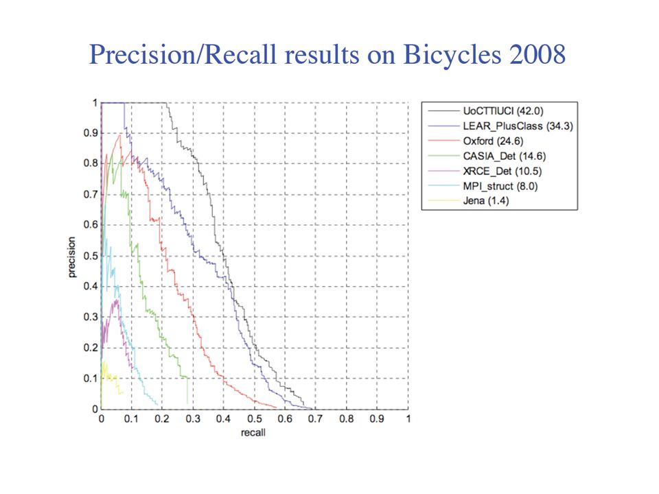
53
All images contain at least 1 bike

55
Future challenges: Dealing with very large number of classes –Imagenet, 15,000 categories, 12 million images To consider: human-level performance for at least one class

Similar presentations


>")


 Each record contains a set of attributes, one of the attributes is the class.>")


 Classification>")

