Download presentation
Presentation is loading. Please wait.

1
Computational Experiments Algorithm run on a Pentium IV 2.4 GHz Instances from “Rete Ferroviaria Italiana” For each station: - minimum interval between 2 arrivals = 4 minutes - minimum interval between 2 departures = 2 minutes Comparison with the currently used “manual” solution

2
Profit of train j = π j – α j v j – β j u j (u j and v j in minutes) Train Typeπjπj αjαj βjβj Eurostar200710 Euronight150710 Intercity12069 Combined11069 Express11058 Direct10058 Local10056 Freight9023 The “shift” and the “stretch” penalties are linear in the shift v j and in the stretch u j, respectively
 Train Typeπjπj αjαj βjβj Eurostar Euronight Intercity12069 Combined11069 Express11058 Direct10058 Local10056 Freight9023 The shift and the stretch penalties are linear in the shift v j and in the stretch u j, respectively")
4
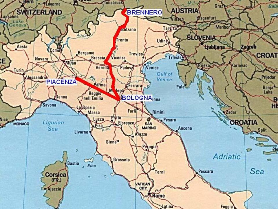
InstanceFirst Station Last Station # stations# trainsIdeal profit PC-BO-aPiacenzaBologna1722125740 PC-BO-bPiacenzaBologna17404800 BRN-BOBrenneroBologna48545470 Characteristics of the instances considered

5
PC-BO-a (221) PC-BO-b (40) BRN-BO (54) Manual Solution Objective function 19830 3181 3332 Scheduled trains 186 32 44 Average shift (minutes) 1.8 4.3 2.0 Average stretch (minutes) 1.6 1.5 2.6 Optimized Solution Objective function 21250 (7.2%) 3593 (13.0%) 4222 (26.7%) Scheduled trains 192 (3.2%) 34 (6.2%) 48 (9.0%) Average shift (minutes) 1.1 (38.8%)3.2 (25.6%)1.2 (40.0%) Average stretch (minutes) 0.5 (68.7%)1.0 (33.3%)1.2 (53.8%) CPU time (seconds) 479 43 59 Results for the basic problem (Lagr. Heur.)
.")
6
Additional Characteristics Fixed block signalling –The line is divided into block sections of predetermined length –Each block section is occupied by at most one train at a time –Short sections are designed to increase line capacity, particularly in high density areas and where speeds are lower Moving block signalling –The position of each train is known continuously by a control center, that takes care of the regulation of the relative distances –Modern technology that requires an efficient communication system between line signals, cabs and control centers

7
PC-BO-a (221) PC-BO-b (40) BRN-BO (54) Manual Solution Objective function 13809 2541 2486 Scheduled trains 127 26 33 Average shift (minutes) 3.9 5.8 4.5 Average stretch (minutes) 1.7 2.5 0.6 Optimized Solution Objective function 15186 (10.0%) 2957 (16.4%) 3075 (23.7%) Scheduled trains 133 (4.7%) 28 (7.7%) 36 (9.0%) Average shift (minutes) 2.0 (48.7%)3.8 (34.5%) 3.2 (28.8%) Average stretch (minutes) 0.9 (47.0%)1.9 (24.0%)0.0 (100.0%) CPU time (seconds) 650.0 29 128 Results with fixed block signalling
 PC-BO-b (40) BRN-BO (54) Manual Solution Objective function Scheduled trains Average shift (minutes) Average stretch (minutes) Optimized Solution Objective function (10.0%) 2957 (16.4%) 3075 (23.7%) Scheduled trains 133 (4.7%) 28 (7.7%) 36 (9.0%) Average shift (minutes) 2.0 (48.7%)3.8 (34.5%) 3.2 (28.8%) Average stretch (minutes) 0.9 (47.0%)1.9 (24.0%)0.0 (100.0%) CPU time (seconds) Results with fixed block signalling")
8
Additional Characteristics (2) Capacities of the Stations The maximim number of trains that can be simultaneously present in each station is given Computational experiments: - capacity = 2 in the major stations - capacity = 1 in the minor stations
 Capacities of the Stations The maximim number of trains that can be simultaneously present in each station is given Computational experiments: - capacity = 2 in the major stations - capacity = 1 in the minor stations")
9
PC-BO-a (221) PC-BO-b (40) BRN-BO (54) Manual Solution Objective function 16806 2784 3252 Scheduled trains 150 27 40 Average shift (minutes) 2.4 4.7 3.1 Average stretch (minutes) 1.4 0.7 0.9 Optimized Solution Objective function 17506 (8.8%) 3291 (18.2%) 4055 (24.7%) Scheduled trains 155 (3.3%) 29 (7.4%) 43 (7.5%) Average shift (minutes) 1.6 (33.3%)2.0 (57.4%)1.4 (19.0%) Average stretch (minutes) 0.6 (57.1%)0.6 (14.3%)0.0 (100.0%) CPU time (seconds) 638 32 167 Results with station capacities
 PC-BO-b (40) BRN-BO (54) Manual Solution Objective function Scheduled trains Average shift (minutes) Average stretch (minutes) Optimized Solution Objective function (8.8%) 3291 (18.2%) 4055 (24.7%) Scheduled trains 155 (3.3%) 29 (7.4%) 43 (7.5%) Average shift (minutes) 1.6 (33.3%)2.0 (57.4%)1.4 (19.0%) Average stretch (minutes) 0.6 (57.1%)0.6 (14.3%)0.0 (100.0%) CPU time (seconds) Results with station capacities")
10
Lagr UB LP UB InstancesValuesecValuesec PC-BO-1 (221,17) 2424367123894814 PC-BO-2 (93,17) 1095379109145 PC-BO-3 (60,17) 72358872005 PC-BO-4 (40,17) 431482409116 MU-VR (54,48) 503257489416 BZ-VR (128,27) 161523151610211 CH-RM (41,102) 5850434582327 BN-BO (68,48) 690914368526 CH-MI (194,16) 212592562113114 MO-MI-1 (16,17) 17272017083
 PC-BO-2 (93,17) PC-BO-3 (60,17) PC-BO-4 (40,17) MU-VR (54,48) BZ-VR (128,27) CH-RM (41,102) BN-BO (68,48) CH-MI (194,16) MO-MI-1 (16,17)")
11
Lagr. Heur. LP Heur InstancesValuesecValuesec PC-BO-1215196712183634489 PC-BO-2108617910882982 PC-BO-37148887151633 PC-BO-436038237792529 MU-VR405514942305612 BZ-VR15993315156225911 CH-RM556043455473963 BN-BO67611436753683 CH-MI207162562097726639 MO-MI-1168420168432

12
Addition of new train paths to an existing timetable (operational scenario) Example: single one-way track Kufstein – Verona: number of stations: 56 (345 km) - number of already scheduled trains: 230 (passenger trains 116, freight trains 114) - time frame period: from 00:00 to 23:59
 Example: single one-way track Kufstein – Verona: number of stations: 56 (345 km) - number of already scheduled trains: 230 (passenger trains 116, freight trains 114) - time frame period: from 00:00 to 23:59")
13
Addition of new freight train paths to an existing timetable (Kufstein- Verona): Example 1) number of requested train paths: 24 (requested departure times with a delay of 5 minutes with respect to an existing path; conflicts among the new paths) maximum shift for each requested train = 10 min maximum stretch = 15 min: # scheduled trains = 11 maximum stretch = 20 min: # scheduled trains = 17 maximum stretch = 25 min: # scheduled trains = 20 maximum stretch = 30 min: # scheduled trains = 22 Running time 18 seconds
: Example 1) number of requested train paths: 24 (requested departure times with a delay of 5 minutes with respect to an existing path; conflicts among the new paths) maximum shift for each requested train = 10 min maximum stretch = 15 min: # scheduled trains = 11 maximum stretch = 20 min: # scheduled trains = 17 maximum stretch = 25 min: # scheduled trains = 20 maximum stretch = 30 min: # scheduled trains = 22 Running time 18 seconds")
14
Addition of new freight train paths to an existing timetable (Kufstein- Verona): Example 2) number of requested train paths: 24 (requested departure times at 00:00, 01:00, …, 23:00) maximum shift for each requested train = 10 min maximum stretch = 15 min: # scheduled trains = 11 maximum stretch = 20 min: # scheduled trains = 15 maximum stretch = 25 min: # scheduled trains = 19 maximum stretch = 30 min: # scheduled trains = 21 Running time 11 seconds
: Example 2) number of requested train paths: 24 (requested departure times at 00:00, 01:00, …, 23:00) maximum shift for each requested train = 10 min maximum stretch = 15 min: # scheduled trains = 11 maximum stretch = 20 min: # scheduled trains = 15 maximum stretch = 25 min: # scheduled trains = 19 maximum stretch = 30 min: # scheduled trains = 21 Running time 11 seconds")
15
Addition of new freight train paths to an existing timetable (Kufstein- Verona): Example 3) number of requested train paths: 48 (requested departure times at 00:00, 00:30, 01:00, …, 23:30) maximum shift for each requested train = 10 min maximum stretch = 15 min: # scheduled trains = 25 maximum stretch = 20 min: # scheduled trains = 33 maximum stretch = 25 min: # scheduled trains = 39 maximum stretch = 30 min: # scheduled trains = 45 Running time 13 seconds
: Example 3) number of requested train paths: 48 (requested departure times at 00:00, 00:30, 01:00, …, 23:30) maximum shift for each requested train = 10 min maximum stretch = 15 min: # scheduled trains = 25 maximum stretch = 20 min: # scheduled trains = 33 maximum stretch = 25 min: # scheduled trains = 39 maximum stretch = 30 min: # scheduled trains = 45 Running time 13 seconds")
16
The considered Railway Network is composed by: the single one-way corridor Kufstein – Verona Porta Nuova the corridor Verona Porta Nuova – Bologna (which presents double- way line segments) the railway node of Bologna the alternative routes from Bologna to Rome (Florence and Falconara) the railway node of Florence the different possible routes from Florence to Rome ( “direttissima”, i.e. the fast line and, “lenta”, i.e. the slow line) the railway node of Rome Railway Network
 the railway node of Rome Railway Network.")
17
We start with a feasible timetable with 679 fixed trains and evaluate two different cases of adding new freight trains: 24 trains, one each hour 48 trains, one each half an hour For both cases, we consider two different possibilities: forbid the alternative slow route (Falconara route) allow to use the slow route (Falconara route) Moreover, we consider different values of the maximum stretch.
 allow to use the slow route (Falconara route) Moreover, we consider different values of the maximum stretch.")
18
The table shows the number of scheduled trains if the Falconara route cannot be used. Name max str 20 minmax str 30 minmax str 45 min 24 trains132122 48 trains294346

19
The table shows the number of scheduled trains if the Falconara route is allowed. Name max str 20 minmax str 30 minmax str 45 min 24 trains162224 48 trains324648

20
Overall Advantages of the Optimization Algorithms Much faster response time with respect to “manual” methods, with the possibility to try several different scenarios Improvement of the solution quality with respect to “manual” methods Satisfaction of a larger number of TO requests Possibility to handle more than one request in “real time”

Similar presentations

 Under Guidance Of Prof. Narayan Rangaraj.>")


 to services that have been proposed in a timetable.>")


 Matteo Fischetti, University of Padua, Italy Double.>")


![3rd ARRIVAL Review Meeting [Patras, 12 May 2009] – WP3 Presentation ARRIVAL – WP3 Algorithms for Robust and online Railway optimization: Improving the.](/16/5057362/big_thumb.jpg "3rd ARRIVAL Review Meeting [Patras, 12 May 2009] – WP3 Presentation ARRIVAL – WP3 Algorithms for Robust and online Railway optimization: Improving the.>")
