Download presentation
Presentation is loading. Please wait.

1
Introduction to R Part 2

2
Working Directory The working directory is where you are currently saving data in R. What is the current working directory? – Type in getwd() – You’ll see the path for your directory Note: I’m using a Mac.
 – You’ll see the path for your directory Note: I’m using a Mac..")
3
Working Directory How to set the working directory: – setwd(“PATH”) If you aren’t really familiar or good with using PATH values, here’s a trick:
 If you aren’t really familiar or good with using PATH values, here’s a trick:")
4
Working Directory Now you can pick the folder you are interested in saving your files to. Once you do that, the bottom right window will show you that folder.

5
Working Directory Why is all this important? – You can use getwd and setwd in saved R scripts to point the analyses to specific files. – Basically, you can set it to import a file from a specific spot and use that over and over, rather than importing the file each time you open R.

6
Packages Packages are add-ons to R that allow you to do different types of analyses, rather than code them yourself. R comes with many pre-programming functions – lovingly called base R. At the top of the help window, you can tell which package a function is included in.

7
Packages Packages are checked/monitored by the CRAN people. – That means there’s some oversight to them. – Many other types of functions can be downloaded from GitHub. Use at your own risk.

8
Packages Note: each time R updates, the packages sometimes come with it, sometimes they don’t. – If you are looking for a specific package, and it doesn’t want to install the normal way (next couple slides), but you know it exists google it and get the TAR files. – You can install them from the TAR files.
, but you know it exists google it and get the TAR files. – You can install them from the TAR files..")
9
Packages How to install: – Console: install.packages(“NAME OF PACKAGE”) – Let’s try it! install.packages(“car”) Note: you have to be connected to the internet for packages to install.
 Note: you have to be connected to the internet for packages to install..")
10
Packages How to install: – Through RStudio – Click on packages, click on install. – Note: you can see here in this window what all you have installed, and if you click on them, you will load that help file (or click the check box to load them).
..")
11
Packages Start typing the name of the package – a drop down will appear with all the options.

12
Packages Now it’s installed! Awesome! That doesn’t mean that it loads every time. – Imagine this: if SPSS had a function that knew how to do regression, but it didn’t load every time. – Annoying! – But this saves computing power by not loading unless you need it. – You will run something without turning on the right package. It’s cool – all the cool kids do it.

13
Packages Packages are also called libraries. You can load them two ways: – In the console: library(car) (look no “” this time). – In the packages window by clicking on the check box.
 (look no this time). – In the packages window by clicking on the check box..")
14
Packages I suggest adding the code to your script to load the packages you need to save yourself the headache of trying to remember which ones were important.

15
Working with Files Data files (like the airquality dataset) come with base R. – You don’t technically have to load them, but you can get them to appear in environment window by: – data(SET NAME)
.")
16
Working with Files If you want to see what’s available, type data() Use the help(DATA SET NAME) or ?DATA SET NAME to see what is included/is part of the data set.
 Use the help(DATA SET NAME) or DATA SET NAME to see what is included/is part of the data set.")
17
Working with Files Data files are not nearly as visual as Excel or SPSS But RStudio can give you somewhat of a visual. – Type View(airquality) to get a visual (note V is capital) – Or click on it in environment window
 to get a visual (note V is capital) – Or click on it in environment window.")
18
Working with Files You can import all types of files, including SPSS files. – I find.csv easiest but that’s me. – You can do.txt with any separator (comma, space, tab)
.")
19
Working with Files Import from Rstudio – Pick your file and click open

20
Working with Files

21
This process is the same as: – real_words <- read.csv(”FILE NAME") – The read.csv function – which has a lot more settings, but this process make it easy to start working with files.
 – The read.csv function – which has a lot more settings, but this process make it easy to start working with files.")
22
Working with Files You can also use the read.table function – which reads more than just csv files, allows you more flexibility in how you import the files.

23
Working with Files Importing SPSS files. – You need the memisc package. as.data.set(spss.system.file(SPSS DATA), use.value.labels=TRUE, to.data.frame=TRUE)
, use.value.labels=TRUE, to.data.frame=TRUE).")
24
Working with Files All of these options will import your data set as a data frame.

25
Working with Files Clear the workspace – You don’t have to do this, but it helps if you want to start over. Click on clear in the environment window. – rm() and remove() functions do the same thing, but you have to type the object names.
 and remove() functions do the same thing, but you have to type the object names..")
26
Functions Functions are pre-written code to help you run analyses (so you don’t have to do the math yourself!). – So there are functions for the mean, variance, z- tests, ANOVA, regression, etc.

27
Functions How to get help on a function (or anything really) – ?function/name/thing – Try ?lm
 – function/name/thing – Try lm")
28
Functions More help on functions: – help(function) – same as ?function – args(function) – tells you all the arguments that the function takes
 – same as function – args(function) – tells you all the arguments that the function takes")
29
Functions What do you mean arguments? Functions have a couple of parts – The name of the function – like lm, mean, var – The arguments – all the pieces inside the () that are required for the function to run.
 that are required for the function to run..")
30
Functions Get help on functions: – example(function) – Gives you an example of the function in action.
 – Gives you an example of the function in action.")
31
Functions Let’s write a very simple function to exponents. You do have to save them, set them equal to something. – pizza = function(x) { x^2 } – You can make more complex function, adding more to the (x) part like (x,y,z). – The variables can be named anything, they just have to match in () and within the {}.
 { x^2 } – You can make more complex function, adding more to the (x) part like (x,y,z). – The variables can be named anything, they just have to match in () and within the {}..")
32
Functions pizza = function(x) { x^2 } – This part is called the formal argument – that’s where you define the function. pizza(2) – The actual argument – that’s where you call the function and use it.
 – The actual argument – that’s where you call the function and use it..")
33
Functions Example functions: – table() – summary() – cov() – cor() – mean() – var() – sd() – scale() – recode()** In car package – relevel() – lower2full() ** Specific to lavaan
 – summary() – cov() – cor() – mean() – var() – sd() – scale() – recode()** In car package – relevel() – lower2full() ** Specific to lavaan")
34
Table Function The table function gives you a frequency table of the values in a vector/column. table(OBJECT NAME)
.")
35
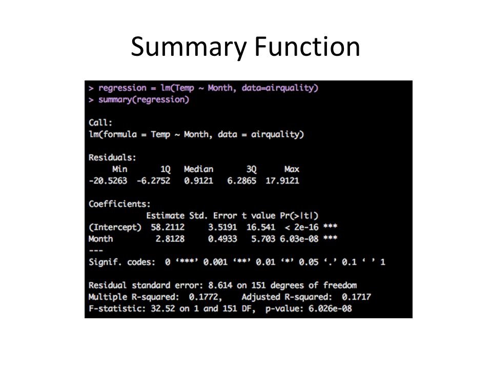
Summary Function The summary function has several uses: – On a vector/data frame, it will give you basic statistics on that information – On a statistical analysis, it will give you the summary output (aka the boxes you are used to looking at in SPSS).
.")
36
Summary Function

38
Descriptives Basic Descriptives – cov() – covariance table – cor() – correlation table – mean() – average – var() – variance – sd() – standard deviation
 – covariance table – cor() – correlation table – mean() – average – var() – variance – sd() – standard deviation")
39
Descriptives Try taking the average of airquality$Ozone mean(airquality$Ozone) – Darn! – Stupid NAs! We’ve talked about how to deal with NAs globally, but here’s how they are handled in functions (generally)
.")
40
Descriptives Try this line instead: – mean(airquality$Ozone, na.rm=TRUE) – Na.rm = remove NAs ?? – The default is FALSE (lame). So you can subset the data or use that argument to tell it to ignore NAs.
. So you can subset the data or use that argument to tell it to ignore NAs..")
41
Descriptives Help / args are your friend**. – The var() function has na.rm – Cov() and cor() do not. **when they are actually helpful that is.
 function has na.rm – Cov() and cor() do not. **when they are actually helpful that is..")
42
Descriptives Try: – cor(airquality, use = “pairwise.complete.obs”)
")
43
Rescoring Functions scale() will mean center or z-score your column. – scale(VARIABLE) Z-scored – scale(VARIABLE, scale=FALSE) Mean centered
 Z-scored – scale(VARIABLE, scale=FALSE) Mean centered.")
44
Rescoring Functions recode() – in the car package, will allow you to reverse code/change the coding of a column – recode(COLUMN/VECTOR, “something=something”)
 – in the car package, will allow you to reverse code/change the coding of a column – recode(COLUMN/VECTOR, something=something )")
45
Rescoring Functions Not quite rescoring, but super handy is – relevel() – Which allows you to change the reference group for dummy coded (factor) variables – relevel(FACTOR, ref=“GROUP NAME”)
 – Which allows you to change the reference group for dummy coded (factor) variables – relevel(FACTOR, ref= GROUP NAME )")
46
Lavaan Package We will use the lower2full function to build covariance matrices to run for SEM. – However, that function is depreciated. – So, use lav_matrix_lower2full(VECTOR OF NUMBERS)
.")
Similar presentations


151 231 2284 CMPDLLM002 Research Methods Lecture 9: Quantitative.>")


 Class #001 (January 9, 2015)>")


