1. The efficient and optimal use of natural resources
chapter 14
The efficient and optimal use of natural resources

2. Objectives
Develop a simple economic model, built around a production function in which natural resources are inputs into the production process;
Identify the conditions that must be satisfied by an economically efficient pattern of natural resource use over time;
Establish the characteristics of a socially optimal pattern of resource use over time in the special case of a utilitarian social welfare function.

3. A simple optimal resource depletion model: the economy and its production function
The economy produces a single good, Q, which can be either consumed or invested.
Consumption increases current well-being, while investment increases the capital stock, permitting greater consumption in the future.
Output is generated through a production function using as inputs a single ‘composite’ non-renewable resource input, R, and manufactured capital, K:
Q = Q(K, R) (14.1)
One possible type of production technology is the Cobb–Douglas (CD) form, consisting of the class of functions
Q = AKαRβ
The production function does not contain labour as a productive input; we have omitted labour to keep the algebra as simple as possible. One could choose to interpret K and R as being in per capita units, so that labour does implicitly enter as a productive input.

4. Is the natural resource essential?
Essentialness of a resource could mean several things.
Here, we interpret this term to mean whether a resource is directly essential for production (where production and the resource are both conceptualised sources at a high degree of aggregation, dealing with general classes such as total output and non-renewable and renewable resources.
A productive input is defined to be essential if output is zero whenever the quantity of that input is zero, irrespective of the amounts of other inputs used. That is, R is essential if Q = Q(K, R = 0) = 0 for any positive value of K.
In the case of the CD production function, R and K are both essential, as setting any input to zero in equation results in Q = 0.
Matters are not so straightforward with the CES function. We state (but without giving a proof) that if θ < 0 then no input is essential, and if θ > 0 then all inputs are essential.

5. Relevance
If we wish to answer questions about the long-run properties of economic systems, the essentialness of non-renewable resources will matter.
Since, by definition, non-renewable resources exist in finite quantities it is not possible to use constant and positive amounts of them over infinite horizons.
However, if a resource is essential, then we know that production can only be undertaken if some positive amount of the input is used.
This seems to suggest that production and consumption cannot be sustained indefinitely if a non-renewable resource is a necessary input to production.
However, if the rate at which the resource is used were to decline asymptotically to zero, and so never actually become zero in finite time, then production could be sustained indefinitely even if the resource were essential.
Whether output could rise, or at least stay constant over time, or whether it would have to decline towards zero will depend upon the extent to which other resources can be substituted for non-renewable resources and upon the behaviour of output as this substitution takes place.

6. Elasticity of substitution
Expression:
or equivalently:
where the partial derivative QR = ∂Q/∂R denotes the marginal product of the resource; QK = ∂Q/∂K denotes the marginal product of capital, and where PR and PK denote the unit prices of the non-renewable resource and capital, respectively.
The elasticity of substitution lies between zero and infinity. Substitution possibilities can be represented diagrammatically. Figure 14.1 shows what are known as production function isoquants. For a given production function, an isoquant is the locus 3 It can also be shown (see Chiang, 1984, for example) that if resources are allocated efficiently in a competitive market economy, the elasticity of substitution between capital and a non-renewable resource is equal to
. That is, the elasticity of substitution measures the proportionate change in the ratio of capital to non-renewable resource used in response to a change in the relative price of the resource to capital.

7. K
 = 0
0 <  < 
The elasticity of substitution lies between zero and infinity.
Substitution possibilities can be represented diagrammatically.
Figure 14.1 shows what are known as production function isoquants. For a given production function, an isoquant is the locus of all combinations of inputs which, when used efficiently, yield a constant level of output.
Given efficient resource use in a competitive economy, the elasticity of substitution measures the proportionate change in the ratio of capital to non-renewable resource used in response to a change in the relative price of the resource to capital.
 =  R
Figure 14.1 Substitution possibilities and the shapes of production function isoquants

8. Substitution possibilities and the shapes of production function isoquants
The differing substitution possibilities are reflected in the curvatures of the isoquants.
In the case where no input substitution is possible (that is, σ = 0), inputs must be combined in fixed proportions and the isoquants will be L-shaped. (Known as Leontief functions. They are commonly used in input–output models of the economy.)
At the other extreme, if substitution is perfect (σ = ), isoquants will be straight lines.
In general, a production function will exhibit an elasticity of substitution somewhere between those two extremes (although not all production functions will have a constant σ for all input combinations). In these cases, isoquants will often be convex to the origin, exhibiting a greater degree of curvature the lower the elasticity of substitution, σ.
For a CES production function, we can also relate the elasticity of substitution to the concept of essentialness. It can be shown that σ = 1/(1 + θ). No input is essential where θ < 0, and all inputs are essential where θ > 0. Given the relationship between σ and θ, it can be seen that no input is essential where σ > 1, and all inputs are essential where σ < 1.
Where σ = 1 (that is, θ = 0), the CES production function collapses to the CD form, where all inputs are essential.

9. Resource substitutability and the consequences of increasing resource scarcity
As production continues throughout time, stocks of non-renewable resources must decline. Continuing depletion of the resource stock will lead to the non-renewable resource price rising relative to the price of capital. As the relative price of the non-renewable resource rises the resource to capital ratio will fall, thereby raising the marginal product of the resource and reducing the marginal product of capital.
However, the magnitude of this substitution effect will depend on the size of the elasticity of substitution. Where the elasticity of substitution is high, only small changes in relative input prices will be necessary to induce a large proportionate change in the quantities of inputs used. ‘Resource scarcity’ will be of little consequence as the economy is able to replace the scarce resource by the reproducible substitute.
Low substitution possibilities mean that as resource depletion pushes up the relative price of the resource, the magnitude of the induced substitution effect will be small. ‘Resource scarcity’ will have more serious adverse effects, as the scope for replacement of the scarce resource by the reproducible substitute is more limited. Where the elasticity of substitution is zero, then no scope exists for such replacement.

10. The feasibility of sustainable development
Is sustainable development actually possible?
To address this question, two things are necessary.
A criterion of sustainability is required.
We need to describe the material transformation conditions available to society, now and in the future. These conditions – the economy’s production possibilities – determine what can be obtained from the endowments of natural and human-made capital over the relevant time horizon.
We adopt here a conventional sustainability criterion: non-declining per capita consumption maintained over indefinite time .
Turning attention to the transformation conditions, it is clear that a large number of factors enter the picture.
What is happening to the size of the human population?
What kinds of resources are available and in what quantities, and what properties do they possess?
What will happen to the state of technology in the future?
How will ecosystems be affected by the continuing waste loads being placed upon the environment, and how will ecosystem changes feed back upon productive potential?

11. Transformation possibilities
To make progress, simplify and narrow down the scope of the problem, by making an assumption about the form of an economy’s production function.
A series of results have become established for several special cases. For the CD and CES functions we have the following.
CASE A: 
Output is produced under fully competitive conditions through a CD production function with constant returns to scale and two inputs, a non-renewable resource, R, and manufactured capital, K, as in the following special case of equation 14.2:
Then, in the absence of technical progress and with constant population, it is feasible to have constant consumption across generations if the share of total output going to capital is greater than the share going to the natural resource (that is, if α > β).
Intuition: For the CD case, although the natural resource is always essential in the sense we described above, if α > β then capital is sufficiently substitutable for the natural resource so that output can be maintained by increasing capital as the depletable resource input diminishes. However, it should be noted that there is an upper bound on the amount of output that can be indefinitely sustained in this case; whether that level is high enough to satisfy ‘survivability’ is another matter.

12. Other cases Case B: Case C:
Output is produced under fully competitive conditions through a CES production function with constant returns to scale and two inputs, a non-renewable resource, R, and manufactured capital, K, as in equation 14.3:
Then, in the absence of technical progress and with constant population, it is feasible to have constant consumption across generations if the elasticity of substitution σ = 1/(1 + θ) is greater than or equal to one.
Case C:
Output is produced under conditions in which a backstop technology is permanently available. In this case, the non-renewable natural resource is not essential. Sustainability is feasible, although there may be limits to the size of the constant consumption level that can be obtained.
For the CES case, if σ > 1, then the resource is not essential. Output can be produced even in the absence of the natural resource.
The fact that the natural resource is finite does not prevent indefinite production (and consumption) of a constant, positive output.
Where σ = 1, the CES production function collapses to the special case of CD, and so Case A applies.
Where a backstop exists (such as a renewable energy source like wind or solar power, or perhaps nuclear-fusion-based power) then it is always possible to switch to that source if the limited natural resource becomes depleted.
We explore this process further in the next chapter.

13. Additional matters
These results assumed that the rate of technical progress and the rate of population growth were both zero.
Results change if one or both of these rates is non-zero.
The presence of permanent technical progress increases the range of circumstances in which indefinitely long-lived constant per capita consumption is feasible.
Constant population growth has the opposite effect.
However, there are circumstances in which constant per capita consumption can be maintained even where population is growing provided the rate of technical progress is sufficiently large and the share of output going to the resource is sufficiently low.
Similarly, for a CES production function, sustained consumption is possible even where σ < 1 provided that technology growth is sufficiently high relative to population growth.
 The general conclusion is that sustainability requires either a relatively high degree of substitutability between capital and the resource, or a sufficiently large continuing rate of technical progress, or the presence of a permanent backstop technology.

14. Sustainability and the Hartwick rule
John Hartwick (1977, 1978): identified two sets of conditions which were sufficient to achieve non-declining consumption through time:
a particular savings rule, known as the Hartwick rule, which states that the rents derived from an efficient extraction programme for the non-renewable resource are invested entirely in reproducible (physical and human) capital;
conditions pertaining to the economy’s production technology, described on a previous slide.
We discuss the implications of the Hartwick rule further in Chapter 19. But three comments about it are worth making at this point.
The Hartwick rule is essentially an ex post description of a sustainable path. Hence if an economy were not already on a sustainable path, then adopting the Hartwick rule is not sufficient for sustainability from that point forwards.
Even were the economy already on a sustainable path, the Hartwick rule requires that the rents be generated from an efficient resource extraction programme in a competitive economy.
Even if the Hartwick rule is pursued subject to this qualification, the savings rule itself does not guarantee sustainability. Technology conditions may rule out the existence of a feasible path.
Comment 1 severely reduces the practical usefulness of the ‘rule’. (See Asheim, 1986, and Pezzey, 1996, and Appendix 19.1 in the present book.)
Comment 3: As we noted in a previous slide, feasibility depends very much upon the extent of substitution possibilities open to an economy.

15. The social welfare function and an optimal allocation of natural resources: model
Social welfare function (SWF)
In general form: (14.5)
where Ut, t = 0,. . ., T, is the aggregate utility in period t.
Assume that the SWF is utilitarian in form:
(14.7)
This defines social welfare as a weighted sum of the utilities of the relevant aggregate of individual persons living at a sequence of points in time.
We assume that utility in each period is a concave function of the level of consumption in that period, so that Ut = U(Ct) for all t, with UC > 0 and UCC < 0.
Notice that the utility function itself is not dependent upon time, so that the relationship between consumption and utility is the same in all periods.
Writing the SWF in this form assumes that it is meaningful to refer to an aggregate level of utility for all individuals in each period. Then social welfare is a function of these aggregates, but not of the distribution of utilities between individuals within each time period. That is a very strong assumption, and by no means the only one we might wish to make. We might justify this by assuming that, for each time period, utility is distributed in an optimal way between individuals.

16. SWF in continuous time form with infinite horizon
For convenience, we switch from discrete-time to continuous-time notation, and assume that the relevant time horizon is infinite.
This leads to the following special case of utilitarian SWF:

17. Constraints Constraint 1: Resource stock-flow constraint
Two constraints that must be satisfied by any optimal solution.
Constraint 1: Resource stock-flow constraint
The resource stock is to be extracted and used by the end of the time horizon.
Given this, together with the fact that we are considering a non-renewable resource for which there is a fixed and finite initial stock, the total use of the resource over time is constrained to be equal to the fixed initial stock.
Denoting the initial stock (at t = 0) as S0 and the rate of extraction and use of the resource at time t as Rt, we can write this constraint as
(14.9 and 14.10)
Equation 14.9 states that the stock remaining at time t (St) is equal to the magnitude of the initial stock (S0) less the amount of the resource extracted over the time interval from zero to t (given by the integral term on the right-hand side of the equation).
Equation has a straightforward interpretation: the rate of depletion of the stock, , is equal to the rate of resource stock extraction, Rt.

18. Second constraint: accounting identity relating consumption, output and the change in the economy’s stock of capital
Output is shared between consumption goods and capital goods, and so that part of the economy’s output which is not consumed results in a capital stock change. Writing this identity in continuous-time form we have:
Given that output is produced through a production function involving two inputs, capital and a non-renewable resource, Qt = Q(Kt, Rt), we can write the constraint as:

19. The optimisation problem

20. First order conditions
Before we discuss the economic interpretations of these equations, it is necessary to explain several things about the notation used and the nature of the solution:
The terms QK (= ∂Q/∂K) and QR (= ∂Q/∂R) are the partial derivatives of output with respect to capital and the non-renewable resource. In economic terms, they are the marginal products of capital and the resource, respectively. Time subscripts are attached to these marginal products to make explicit the fact that their values will vary over time in the optimal solution.
The terms Pt and ωt are the shadow prices of the two productive inputs, the natural resource and capital. These two variables carry time subscripts because the shadow prices will vary over time. The solution values of Pt and ωt, for t = 0, 1, . . ., , define optimal time paths for the prices of the natural resource and capital.6
The quantity being maximised in equation 14.8 is a sum of (discounted) units of utility. Hence the shadow prices are measured in utility, not consumption (or money income), units. You should now turn to Box 14.2 where an explanation of the relationship between prices in utils and prices in consumption (or income) units is given.
6 A shadow price is a price that emerges as a solution to an optimisation problem; put another way, it is an implicit or ‘planning’ price that a good (or in this case, a productive input) will take if resources are allocated optimally over time. If an economic planner were using the price mechanism to allocate resources over time, then {Pt} and {ωt}, t = 0, 1, .. ., , would be the prices he or she should establish in order to achieve an efficient and optimal resource allocation.
QK (= ∂Q/∂K) and QR (= ∂Q/∂R) are the partial derivatives of output with respect to capital and the non-renewable resource. (i.e. the marginal products of capital and the resource).
Time subscripts are attached to these marginal products to make explicit the fact that their values will vary over time in the optimal solution.
The terms Pt and ωt are the shadow prices of the two productive inputs, the natural resource and capital. These two variables carry time subscripts because the shadow prices will vary over time. The solution values of Pt and ωt, for t = 0, 1, . . ., , define optimal time paths for the prices of the natural resource and capital.
The quantity being maximised in equation 14.8 is a sum of (discounted) units of utility. Hence the shadow prices are measured in utility, not consumption (or money income), units.

21. First order conditions
Equation 14.14a: In each period, the marginal utility of consumption UC,t must be equal to the shadow price of capital ωt . An efficient outcome will be one in which the marginal net benefit of using one unit of output for consumption is equal to its marginal net benefit when it is added to the capital stock.

22. First order conditions
Equation 14.14b: The value of the marginal product of the natural resource must be equal to the marginal value (or shadow price) of the natural resource stock, Pt. The value of the marginal product of the resource is the marginal product in units of output (QR,t) multiplied by the value of one unit of output(, ωt).

23. Static and dynamic efficiency conditions
The static efficiency conditions
As with any asset, static efficiency requires that, in each use to which a resource is put, the marginal value of the services from it should be equal to the marginal value of that resource stock in situ. This ensures that the marginal net benefit (or marginal value) to society of the resource should be the same in all its possible uses.
This is what equations 14.14a and 14.14b imply.
Equation 14.14a: In each period, the marginal utility of consumption UC,t must be equal to the shadow price of capital ωt . An efficient outcome will be one in which the marginal net benefit of using one unit of output for consumption is equal to its marginal net benefit when it is added to the capital stock.
Equation 14.14b: The value of the marginal product of the natural resource must be equal to the marginal value (or shadow price) of the natural resource stock, Pt. The value of the marginal product of the resource is the marginal product in units of output (QR,t) multiplied by the value of one unit of output(, ωt).
Equation 14.14a. This states that, in each period, the marginal utility of consumption UC,t must be equal to the shadow price of capital ωt (remembering that prices are measured in units of utility here). A marginal unit of output can be used for consumption now (yielding UC,t units of utility) or added to the capital stock (yielding an amount of capital value ωt in utility units). An efficient outcome will be one in which the marginal net benefit of using one unit of output for consumption is equal to its marginal net benefit when it is added to the capital stock.
Equation 14.14b states that the value of the marginal product of the natural resource must be equal to the marginal value (or shadow price) of the natural resource stock. This shadow price is, of course, Pt. The value of the marginal product of the resource is the marginal product in units of output (i.e. QR,t) multiplied by the value of one unit of output, ωt. But we have defined ωt as the price of a unit of capital; so why is this the value of one unit of output? The reason is simple. In this economy, units of output and units of capital are in effect identical (along an optimal path). Any output that is not consumed is added to capital. So we can call ωt either the value of a marginal unit of capital or the value of a marginal unit of output.

24. The dynamic efficiency conditions
Dynamic efficiency requires that each asset or resource earns the same rate of return, and that this rate of return is the same at all points in time, being equal to the social rate of discount.
Equations 14.14c and 14.14d ensure that dynamic efficiency is satisfied.
Equation 14.14c: Dividing each side by P we obtain which states that the growth rate of the shadow price of the natural resource (that is, its own rate of return) should equal the social utility discount rate.
Equation 14.14d: Dividing both sides of 14.14d by ω, we obtain an expression which states that the return to physical capital (its capital appreciation plus its marginal productivity) must equal the social discount rate.

25. First order conditions
Equation 14.14c: Dividing each side by P the expression states that the growth rate of the shadow price of the natural resource (that is, its own rate of return) should equal the social utility discount rate.

26. First order conditions
Equation 14.14d: Dividing both sides of 14.14d by ω, we obtain an expression
which states that the return to physical capital (its capital appreciation plus its marginal productivity) must equal the social discount rate.

27. Hotelling’s rule: two interpretations
Equation 14.14c is known as Hotelling’s rule for the extraction of non-renewable resources. It is often expressed in the form
(14.15)
The Hotelling rule is an intertemporal efficiency condition which must be satisfied by any efficient process of resource extraction.
A few lines of algebra ( given in the text) yields the following expression:
which give a second interpretation: the discounted price of the natural resource is constant along an efficient resource extraction path.
In other words, Hotelling’s rule states that the discounted value of the resource should be the same at all dates. But this is merely a special case of a general asset–efficiency condition; the discounted (or present value) price of any efficiently managed asset will remain constant over time. This way of interpreting Hotelling’s rule shows that there is nothing special about natural resources per se when it comes to thinking about efficiency. A natural resource is an asset. All efficiently managed assets will satisfy the condition that their discounted prices should be equal at all points in time. If we had wished to do so, the Hotelling rule could have been obtained directly from this general condition.

28. Hotelling’s rule: an implication
Note the effect of changes in the social discount rate on the optimal path of resource price.
The higher is ρ, the faster should be the rate of growth of the natural resource price.

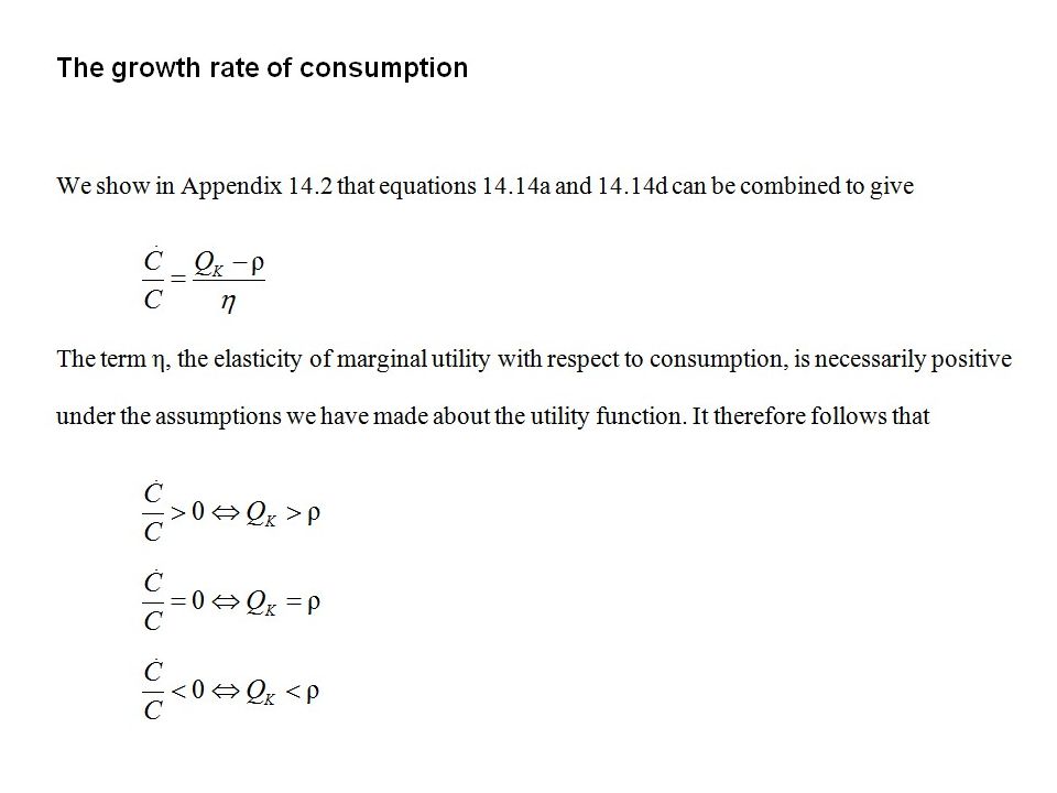
30. Intuition
The social discount rate, ρ, reflects impatience for future consumption
QK (the marginal product of capital) is the pay-off to delayed consumption.
The relations imply that along an optimal path:
consumption is increasing when ‘pay-off’ is greater than ‘impatience’;
consumption is constant when ‘pay-off’ is equal to ‘impatience’;
consumption is decreasing when ‘pay-off’ is less than ‘impatience’.
Therefore, consumption is growing over time along an optimal path if the marginal product of capital (QK) exceeds the social discount rate (ρ); consumption is constant if QK = ρ; and consumption growth is negative if the marginal product of capital is less than the social discount rate. This makes sense, given that:
when ‘pay-off’ is greater than ‘impatience’, the economy will be accumulating K and hence growing;
when ‘pay-off’ and ‘impatience’ are equal, K will be constant;
when ‘pay-off’ is less than ‘impatience’, the economy will be running down K.

31. Figure 14.2 The logarithmic utility function

32. Figure 14.3 Two price paths, each satisfying Hotelling’s rulePt
PtB = P0Bet
PtA = P0Aet
Optimality in resource extraction
The astute reader will have noticed that we have described the Hotelling rule (and the other conditions described above) as an efficiency condition. But a rule that requires the growth rate of the price of a resource to be equal to the social discount rate does not give rise to a unique price path. This should be evident by inspection of Figure 14.3, in which two different initial prices, say 1 util and 2 utils, grow over time at the same discount rate, say 5%. If ρ were equal to 5%, each of these paths – and indeed an infinite quantity of other such price paths – satisfies Hotelling’s rule, and so they are all efficient paths. But only one of these price paths can be optimal, and so the Hotelling rule is a necessary but not a sufficient condition for optimality.
How do we find out which of all the possible efficient price paths is the optimal one? An optimal solution requires that all of the conditions listed in equations 14.14a–d, together with initial conditions relating to the stocks of capital and resources and terminal conditions (how much stocks, if any, should be left at the terminal time), are satisfied simultaneously. So Hotelling’s rule – one of these conditions – is a necessary but not sufficient condition for an optimal allocation of natural resources over time.
Let us think a little more about the initial and final conditions for the natural resource that must be satisfied. There will be some initial resource stock; similarly, we know that the resource stock must converge to zero as elapsed time passes and the economy approaches the end of its planning horizon. If the initial price were ‘too low’, then this would lead to ‘too large’ amounts of resource use in each period, and all the resource stock would become depleted in finite time (that is, before the end of the planning horizon). Conversely, if the initial price were ‘too high’, then this would lead to ‘too small’ amounts of resource use in each period, and some of the resource stock would (wastefully) remain undepleted at the end of the planning horizon. This suggests that there is one optimal initial price that would bring about a path of demands that is consistent with the resource stock just becoming fully depleted at the end of the planning period.
In conclusion, we can say that while equations are each efficiency conditions, taken jointly as a set (together with initial values for K and S) they implicitly define an optimal solution to the optimisation problem, by yielding unique time paths for Kt and Rt and their associated prices that maximise the social welfare function.
P0B
P0A
time, t

33. Extending the model to incorporate extraction costs
Modelling extraction costs
Denote total extraction costs as ; the amount of the resource being extracted as R; and remaining resource stock as S.
We would expect that  will be an increasing function of R. Also, in many circumstances, costs will depend on the size of the remaining stock of the resource, typically rising as the stock becomes more depleted.
Letting St denote the size of the resource stock at time t (the amount remaining after all previous extraction) we can write extraction costs as
(14.19)

34. t (for given value of Rt = )
Figure 14.4 Three possible examples of the relationship between extraction costs and remaining stock for a fixed level of resource extraction, R
t (for given value of Rt = )
(iii)
(ii)
(i)
The relationship denoted (i) corresponds to the case where the total extraction cost is independent of the stock size. In this case, the extraction cost function collapses to the simpler form t = 1(Rt) in which extraction costs depend only on the quantity extracted per period of time.
In case (ii), the costs of extracting a given quantity of the resource increase linearly as the stock becomes increasingly depleted. S = ∂/∂S is then a constant negative number.
Finally, case (iii) shows the costs of extracting a given quantity of the resource increasing at an increasing rate as S falls towards zero; S is negative but not constant, becoming larger in absolute value as the resource stock size falls. This third case is the most likely one for typical non-renewable resources. S0
Remaining resource stock, St

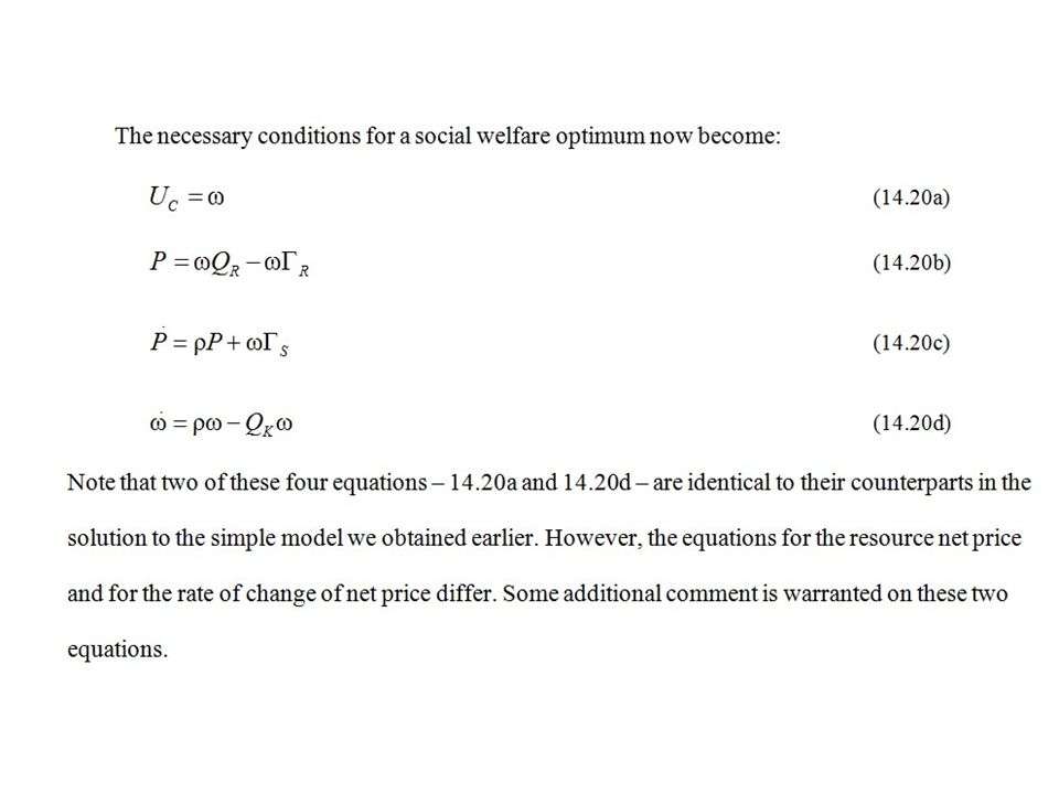
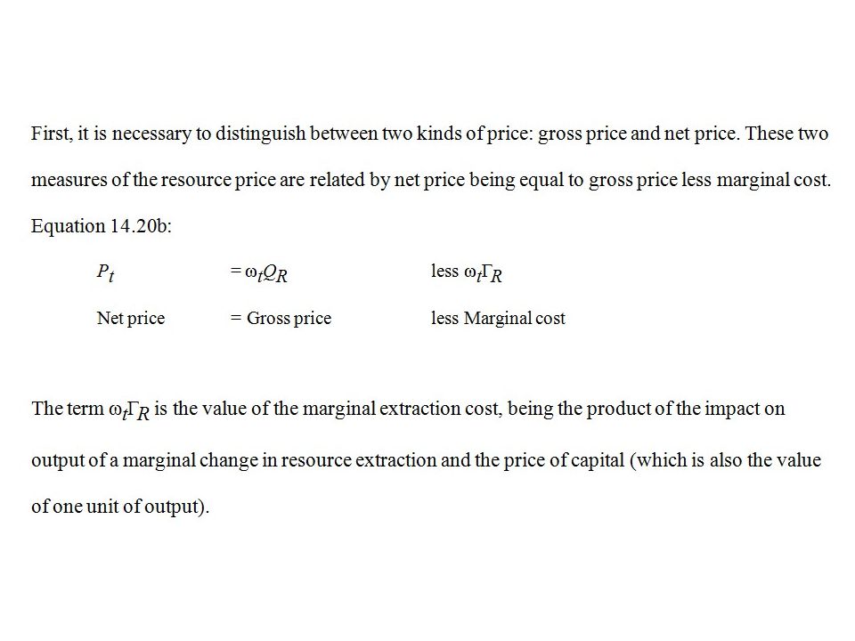
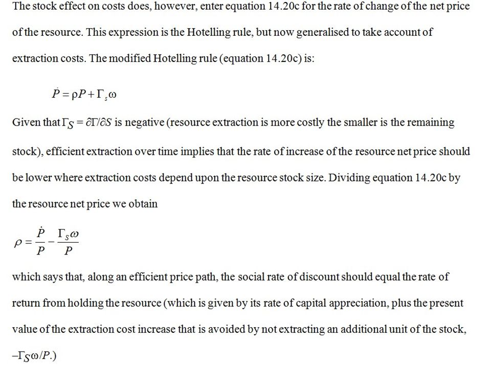
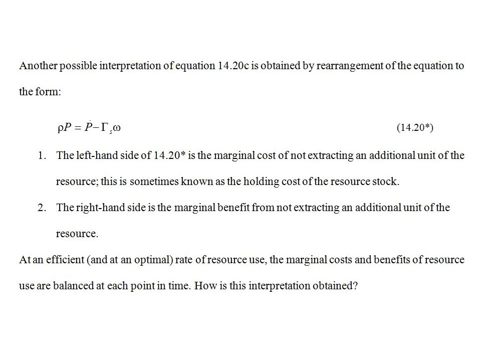
35. The optimal solution to the resource depletion model incorporating extraction costs

40. Conclusion
The presence of costs related to the level of resource extraction raises the gross price of the resource above its net price but has no effect on the growth rate of the resource net price.
In contrast, a resource stock size effect on extraction costs will slow down the rate of growth of the resource net price.
In most circumstances, this implies that the resource net price has to be higher initially (but lower ultimately) than it would have been in the absence of this stock effect. As a result of higher initial prices, the rate of extraction will be slowed down in the early part of the time horizon, and a greater quantity of the resource stock will be conserved (to be extracted later).

41. Generalisation to renewable resources
Only brief comment here as lengthy analysis of the allocation of renewable resources covered in Chapters 17 and 18.
Assume that the amount of natural growth of non-renewable resources, Gt, is some function of the current stock level, so that Gt = G(St).
Then write the relationship between the change in the resource stock and the rate of extraction (or harvesting) of the resource as
(14.21)

42. Generalisation to renewable resources (2)
The efficiency conditions required by an optimal allocation of resources are now different from the case of non-renewable resources.
However, a modified version of the Hotelling rule for rate of change of the net price of the resource still applies, given by
Inspection of this modified Hotelling rule for renewable resources demonstrates that the rate at which the net price should change over time depends upon GS, the rate of change of resource growth with respect to changes in the stock of the resource.

43. Steady-state harvesting
A steady-state harvesting of a renewable resource exists when all stocks and flows are constant over time.
In particular, a steady-state harvest will be one in which the harvest level is fixed over time and is equal to the natural amount of growth of the resource stock.
Additions to and subtractions from the resource stock are thus equal, and the stock remains at a constant level over time.
If demand for the resource is constant over time, the resource net price will remain constant in a steady state, as the quantity harvested each period is constant.
In a steady state, the Hotelling rule simplifies to
ρP = PGS (14.23)
and so
ρ = GS (14.24)

44. Figure 14.5 The relationship between the resource stock size, S, and the growth of the resource, G
MSY = GMAX G*
It is common to assume that the relationship between the resource stock size, S, and the growth of the resource, G, is as indicated in Figure This relationship is explained more fully in Chapter 17.
As the stock size increases from zero, the amount of growth of the resource rises, reaches a maximum, known as the maximum sustainable yield (MSY), and then falls. Note that GS = dG/dS is the slope at any point of the growth–stock function in Figure 14.5. S* S

45. Complications & extensions
The model set up assumes that there is a single, known, finite stock of a non-renewable resource. Furthermore, the whole stock was assumed to have been homogeneous in quality. In practice, both of these assumptions are often false.
The following situations are likely:
The total stock is not known with certainty.
New discoveries increase the known stock of the resource.
A distinction needs to be drawn between the physical quantity of the stock and the economically viable stock size.
Research and development, and technical progress, take place, which can change extraction costs, the size of the known resource stock, the magnitude of economically viable resource deposits, and estimates of the damages arising from natural resource use.
Even when we focus on a particular kind of non-renewable resource, the stock is likely to be heterogeneous. Different parts of the total stock are likely to be uneven in quality, or to be located in such a way that extraction costs differ for different portions of the stock.

46. Backstop technology
By treating all non-renewable resources as one composite good, our analysis in this chapter had no need to consider substitutes for the resource in question (except, of course, substitutes in the form of capital and labour).
But once our analysis enters the more complex world in which there are a variety of different non-renewable resources which are substitutable for one another to some degree, analysis inevitably becomes more complicated.
One particular issue of great potential importance is the presence of backstop technologies (see Chapter 15).
The existence of a backstop technology will set an upper limit on the level to which the price of a resource can go. If the cost of the ‘original’ resource were to exceed the backstop cost, users would switch to the backstop.
Suppose that we are currently using some non-renewable resource for a particular purpose – perhaps for energy production. It may well be the case that another resource exists that can substitute entirely for the resource we are considering, but may not be used at present because its cost is relatively high. Such a resource is known as a backstop technology. For example, renewable power sources such as wind energy are backstop alternatives to fossil-fuel-based energy.