Download presentation
Presentation is loading. Please wait.

1
Copyright © 2005. The McGraw-Hill Companies, Inc. Permission required for reproduction or display. Introduction to MATLAB 7 for Engineers William J. Palm III Chapter 1 An Overview Of MATLAB PowerPoint to accompany

2
Matlab's capabilities Hard to describe, best shown with user stories: http://www.mathworks.com/company/user_sto ries/ Hard to describe, best shown with user stories: http://www.mathworks.com/company/user_sto ries/ http://www.mathworks.com/company/user_sto ries/ http://www.mathworks.com/company/user_sto ries/ basically takes the tedium out of doing complex, specialized, math calculations basically takes the tedium out of doing complex, specialized, math calculations some programs like MathCad help you "do math" some programs like MathCad help you "do math" Matlab is more a "Problem solving" tool. Matlab is more a "Problem solving" tool. Simulation, Verify speculative possibilities Simulation, Verify speculative possibilities Combined with programming language for extensibility Combined with programming language for extensibility

3
The default MATLAB Desktop. Figure 1.1–1 1-2 More? See pages 6-7.

4
Entering Commands and Expressions MATLAB retains your previous keystrokes. Use the up-arrow key to scroll back back through the commands. Press the key once to see the previous entry, and so on. Use the down-arrow key to scroll forward. Edit a line using the left- and right-arrow keys the Backspace key, and the Delete key. Press the Enter key to execute the command. 1-3

5
An Example Session >> 8/10 ans = 0.8000 >> 5*ans ans = 4 >> r=8/10 r = 0.8000 >> r r = 0.8000 >> s=20*r s = 16 1-4 More? See pages 8-9.

6
Scalar Arithmetic Operations Table 1.1–1 1-5 Symbol Operation MATLAB form ^ exponentiation: a b a^b * multiplication: ab a*b / right division: a/b a/b \ left division: b/a a\b + addition: a + b a + b - subtraction: a - b a - b

7
Order of Precedence Table 1.1–2 1-6 Precedence Operation FirstParentheses, evaluated starting with the innermost pair. SecondExponentiation, evaluated from left to right. ThirdMultiplication and division with equal precedence, evaluated from left to right. FourthAddition and subtraction with equal precedence, evaluated from left to right.

8
Examples of Precedence >> 8 + 3*5 ans = 23 >> 8 + (3*5) ans = 23 >>(8 + 3)*5 ans = 55 >>4^212 8/4*2 ans = 0 >>4^212 8/(4*2) ans = 3 1-7 (continued …)
 ans = 23 >>(8 + 3)*5 ans = 55 >>4^212 8/4*2 ans = 0 >>4^212 8/(4*2) ans = (continued …)")
9
Examples of Precedence (continued) >> 3*4^2 + 5 ans = 53 >>(3*4)^2 + 5 ans = 149 >>27^(1/3) + 32^(0.2) ans = 5 >>27^(1/3) + 32^0.2 ans = 5 >>27^1/3 + 32^0.2 ans = 11 1-8
 >> 3*4^2 + 5 ans = 53 >>(3*4)^2 + 5 ans = 149 >>27^(1/3) + 32^(0.2) ans = 5 >>27^(1/3) + 32^0.2 ans = 5 >>27^1/3 + 32^0.2 ans =")
10
The Assignment Operator = Typing x = 3 assigns the value 3 to the variable x. Typing x = 3 assigns the value 3 to the variable x. We can then type x = x + 2. This assigns the value 3 + 2 = 5 to x. But in algebra this implies that 0 = 2. We can then type x = x + 2. This assigns the value 3 + 2 = 5 to x. But in algebra this implies that 0 = 2. In algebra we can write x + 2 = 20, but in MATLAB we cannot. In algebra we can write x + 2 = 20, but in MATLAB we cannot. In MATLAB the left side of the = operator must be a single variable. In MATLAB the left side of the = operator must be a single variable. The right side must be a computable value. The right side must be a computable value. 1-9 More? See pages 11-12.

11
Commands for managing the work session Table 1.1–3 1-10 CommandDescription clc Clears the Command window. clear Removes all variables from memory. clear v1 v2 Removes the variables v1 and v2 from memory. exist(‘var’) Determines if a file or variable exists having the name ‘ var ’. quit Stops MATLAB. (continued …)
 Determines if a file or variable exists having the name ‘ var ’. quit Stops MATLAB. (continued …).")
12
Commands for managing the work session Table 1.1–3 (continued) who Lists the variables currently in memory. whos Lists the current variables and sizes, and indicates if they have imaginary parts. ;Semicolon; suppresses screen printing; also denotes a new row in an array. 1-11More? See pages 12-15.

13
Special Variables and Constants Table 1.1–4 1-12 Command Description ans Temporary variable containing the most recent answer. eps Specifies the accuracy of floating point precision. i,j The imaginary unit 1. Inf Infinity. NaN Indicates an undefined numerical result. pi The number .

14
Complex Number Operations The number c 1 = 1 – 2i is entered as follows: c1 = 12i. An asterisk is not needed between i or j and a number, although it is required with a variable, such as c2 = 5 i*c1. Be careful. The expressions y = 7/2*i and x = 7/2i give two different results: y = (7/2)i = 3.5i and x = 7/(2i) = –3.5i. 1-13
i = 3.5i and x = 7/(2i) = –3.5i")
15
Numeric Display Formats Table 1.1–5 1-14 Command Description and Example format short Four decimal digits (the default); 13.6745. format long 16 digits; 17.27484029463547. format short e Five digits (four decimals) plus exponent; 6.3792e+03. format long e 16 digits (15 decimals) plus exponent; 6.379243784781294e–04.
 plus exponent; e+03. format long e 16 digits (15 decimals) plus exponent; e–04..")
16
Some Commonly Used Mathematical Functions Table 1.3–1 1-18 Function MATLAB syntax 1 e x exp(x) √x sqrt(x) ln x log(x) log 10 x log10(x) cos x cos(x) sin x sin(x) tan x tan(x) cos 1 x acos(x) sin 1 x asin(x) tan 1 x atan(x) 1 The MATLAB trigonometric functions use radian measure.
 √x sqrt(x) ln x log(x) log 10 x log10(x) cos x cos(x) sin x sin(x) tan x tan(x) cos 1 x acos(x) sin 1 x asin(x) tan 1 x atan(x) 1 The MATLAB trigonometric functions use radian measure.")
17
Arrays The numbers 0, 0.1, 0.2, …, 10 can be assigned to the variable u by typing u = [0:0.1:10]. To compute w = 5 sin u for u = 0, 0.1, 0.2, …, 10, the session is; >>u = [0:0.1:10]; >>w = 5*sin(u); The single line, w = 5*sin(u), computed the formula w = 5 sin u 101 times. 1-15
![Arrays The numbers 0, 0.1, 0.2, …, 10 can be assigned to the variable u by typing u = [0:0.1:10].](http://images.slideplayer.com/24/7324729/slides/slide_17.jpg "To compute w = 5 sin u for u = 0, 0.1, 0.2, …, 10, the session is; >>u = [0:0.1:10]; >>w = 5*sin(u); The single line, w = 5*sin(u), computed the formula w = 5 sin u 101 times")
18
Problem Solving The point of learning Matlab is to help us solve problems in Engineering,Science,Math The point of learning Matlab is to help us solve problems in Engineering,Science,Math Matlab is just a tool—it won't think for us Matlab is just a tool—it won't think for us We still need to apply the engineering problem solving method We still need to apply the engineering problem solving method Much of our thought process needs to take place "offline" i.e. using traditional sketches and paper based mathematics Much of our thought process needs to take place "offline" i.e. using traditional sketches and paper based mathematics Computer tools require special care to make sure the answers are correct Computer tools require special care to make sure the answers are correct

19
Steps in engineering problem solving Table 1.7–1 1. 1. Understand the purpose of the problem. 2. 2. Collect the known information. Realize that some of it might later be found unnecessary. 3. 3. Determine what information you must find. 4. 4. Simplify the problem only enough to obtain the required information. State any assumptions you make. 5. 5. Draw a sketch and label any necessary variables. 6. 6. Determine which fundamental principles are applicable. 7. 7. Think generally about your proposed solution approach and consider other approaches before proceeding with the details. (continued …) 1-56
")
20
Steps in engineering problem solving Table 1.7–1 (continued) 8. Label each step in the solution process. Understand the purpose of the problem 9. If you solve the problem with a program, hand check the results using a simple version of the problem. Checking the dimensions and units and printing the results of intermediate steps in the calculation sequence can uncover mistakes. (continued …) 1-57
")
21
Steps in engineering problem solving Table 1.7–1 (continued) 10. Perform a “reality check” on your answer. Does it make sense? Estimate the range of the expected result and compare it with your answer. Do not state the answer with greater precision than is justified by any of the following: (a)The precision of the given information. (b)The simplifying assumptions. (c)The requirements of the problem. Interpret the mathematics. If the mathematics produces multiple answers, do not discard some of them without considering what they mean. The mathematics might be trying to tell you something, and you might miss an opportunity to discover more about the problem. 1-58More? See pages 52-56.
The precision of the given information. (b)The simplifying assumptions. (c)The requirements of the problem. Interpret the mathematics. If the mathematics produces multiple answers, do not discard some of them without considering what they mean. The mathematics might be trying to tell you something, and you might miss an opportunity to discover more about the problem. 1-58More. See pages")
22
Steps for developing a computer solution Table 1.7–2 1. 1. State the problem concisely. 2. 2. Specify the data to be used by the program. This is the “input.” 3. 3. Specify the information to be generated by the program. This is the “output.” 4. 4. Work through the solution steps by hand or with a calculator; use a simpler set of data if necessary. 5. 5. Write and run the program. 6. 6. Check the output of the program with your hand solution. 7. 7. Run the program with your input data and perform a reality check on the output. 8. 8. If you will use the program as a general tool in the future, test it by running it for a range of reasonable data values; perform a reality check on the results. 1-59More? See pages 56-60.

23
23 Rev.S08 How to Solve an Applied Trigonometry Problem? Step 1Draw a sketch, and label it with the given information. Label the quantity to be found with a variable. Step 2Use the sketch to write an equation relating the given quantities to the variable. Step 3Solve the equation, and check that your answer makes sense.

24
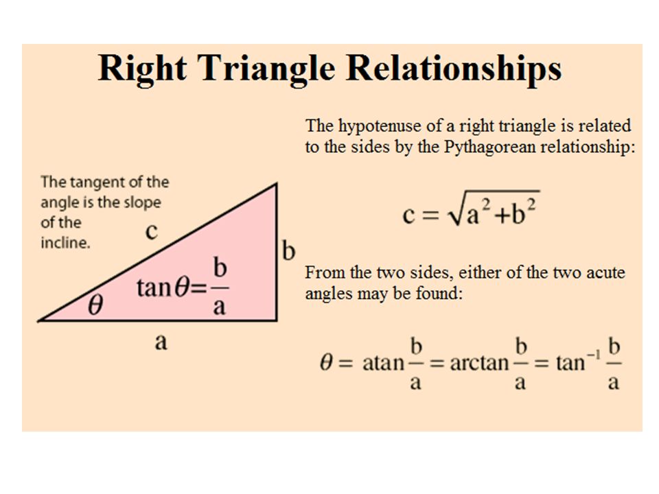
Laws of Trig you should Master Pythagorean theorem: a 2 +b 2 =c 2 (right triangles) Sum of internal angles = 180 (all triangles) Definition of sin, cos, tan, arcsin, arccos, arctan (right triangles) Law of Cosines (all triangles) Law of Sines (all triangles)
 Sum of internal angles = 180 (all triangles) Definition of sin, cos, tan, arcsin, arccos, arctan (right triangles) Law of Cosines (all triangles) Law of Sines (all triangles)")
26
Defining sin, cos, tan also, a = c cos( ), b = c sin( ) = arccos(a/ c) = arcsin(b/c) = arctan(b/a)
, b = c sin( ) = arccos(a/ c) = arcsin(b/c) = arctan(b/a)")
27
27 Rev.S08 Example http://faculty.valenciacc.edu/ashaw/ Click link to download other modules. The length of the shadow of a tree 22.02 m tall is 28.34 m. Find the angle of elevation of the sun. Draw a sketch. The angle of elevation of the sun is 37.85 . 22.02 m 28.34 m B

28
28 Rev.S08 Example 2 http://faculty.valenciacc.edu/ashaw/ Click link to download other modules. The length of the shadow of a tree is 100 ft, and the angle of elevation of the sun is 60 degrees. Find the height of the tree: 100 = hyp*cos(60), therefore hyp = 100/cos(60) = 200 height = hyp*sin(60) = 200*.866 = 173 ft
, therefore hyp = 100/cos(60) = 200 height = hyp*sin(60) = 200*.866 = 173 ft.")
29
Law of Cosines Use when you know an angle and two adacent sides to find the 3 rd side Use when you know three sides and want to find an angle

30
Find x Matlab: x = sqrt(14^2+10^2-2*14*10*cosd(44)) = 9.725 (use cosd for degree angles)
) = (use cosd for degree angles)")
31
Find x paper: 25 2 = 37 2 + 32 2 – 2*37*32*cos(x) cos(x) = (37 2 + 32 2 – 25 2 ) / (2*37*32) Matlab: x = acosd((37 2 + 32 2 – 25 2 ) / (2*37*32) )
 cos(x) = ( – 25 2 ) / (2*37*32) Matlab: x = acosd(( – 25 2 ) / (2*37*32) )")
32
Law of Sines Use when you know an angle and the opposite side and want to find another angle or side:

33
Find b (paper) sin(b)/16 = sin(115)/123 (matlab) b = asind( 16*sind(115)/123) = 6.77 deg (use sind for degrees)
 sin(b)/16 = sin(115)/123 (matlab) b = asind( 16*sind(115)/123) = 6.77 deg (use sind for degrees)")
34
U Try: Find unknown side x a x (paper) (matlab)
 (matlab)")
Similar presentations


, Data Analysis,>")


 Is a solution to ? B) Is a solution to cos x = sin 2x ?>")


. (2). (3). There are 10 boys and 12 girls in a Math 2 class. Write the ratio of the number of girls to the number.>")


