1. Trapped Atomic Ions II Scaling the Ion Trap Quantum Computer Christopher Monroe FOCUS Center & Department of Physics University of Michigan

4. Universal Quantum Logic Gates with Trapped Ions Step 1 Laser cool collective motion to rest Cirac and Zoller, Phys. Rev. Lett. 74, 4091 (1995) n=0

5. Universal Quantum Logic Gates with Trapped Ions laser j k Step 2 Map j th qubit to collective motion Cirac and Zoller, Phys. Rev. Lett. 74, 4091 (1995)

6. Universal Quantum Logic Gates with Trapped Ions laser j k Step 3 Flip k th qubit depending upon motion Cirac and Zoller, Phys. Rev. Lett. 74, 4091 (1995)

7. Universal Quantum Logic Gates with Trapped Ions laser j k Step 4 Remap collective motion to j th qubit (reverse of Step 1) Cirac and Zoller, Phys. Rev. Lett. 74, 4091 (1995) Net result: [| j + | j ] | k  | j | k + | j | k n=0

9. Four-qubit quantum logic gate Sackett, et al., Nature 404, 256 (2000) |   |  + e i  | 

10.  =  m +  m During the gate (at some point), the state of an ion qubit and motional bus state is: Decoherence Kills the Cat

11. Anomalous heating in ion traps Q. Turchette, et. al., Phys. Rev. A 61, 063418-8 (2000) L. Deslauriers et al., Phys. Rev. A 70, 043408 (2004) Heating due to fluctuating patch potentials (?) ~ 1/d 4 d

12. 0.040.10.20.30.6 10 -2 10 10 0 1 2 S E (  )  10 -12 (V/m) 2 /Hz 40 Ca + 199 Hg + 111 Cd + 137 Ba + 9 Be + 1/d 4 guide-to-eye Electric Field Noise History in 3-6 MHz traps est. thermal noise Distance to nearest trap electrode [mm] Q. Turchette, et. al., Phys. Rev. A 61, 063418-8 (2000) L. Deslauriers et al., Phys. Rev. A 70, 043408 (2004) 137 Ba + IBM-Almaden (2002) 40 Ca + Innsbruck (1999) 199 Hg + NIST (1989) 9 Be + NIST (1995-) 111 Cd + Michigan (2003)

14. 0.3 mm J. Bergquist, NIST ion loading? ion lifetime?

16. Photoionization-loading of Cd + into trap Cd + loading rate (sec -1 ) laser center wavelength (nm) Cd 1 S 0  1 P 1 transition (a)Off-resonant 266nm 10Hz nsec YAG (b) Resonant 229nm 80 MHz psec Ti:Saph (P avg 1 mW) 228.4228.6228.8229.0229.2229.4 0 1 2 3 laser bandwidth 1S01S0 1P11P1 continuum 229nm Neutral Cd

17. + E(r) ? Ion Trap Tricks to “get around”  E  : (1)Apply magnetic field along z; ev  B Lorentz force confines in xy plane PENNING TRAP  large capacity (1-10 8 )  ions rotate around z  confinement limited by eB/mc + E(r) NO!  E  quadrupole: E(r) =  (x + y  2z) z

18. ~few 1000 Be + ions in a Penning Trap J. Bollinger, NIST Quantum Hard-drive?

19. + E(r) ? Ion Trap Tricks to “get around”  E  : (1)Apply magnetic field along z; ev  B Lorentz force confines in xy plane PENNING TRAP  large capacity (1-10 8 )  ions rotate around z  confinement limited by eB/mc + E(r) NO!  E  quadrupole: E(r) =  (x + y  2z) z W. Paul H. Dehmelt (2) Apply sinusoidal electric quadrupole field RF (PAUL) TRAP  ions stationery (on average)  strong confinement sin  t

21. x + [  2 cos  t]x = 0  Dynamics of a single ion in a rf trap time position x “secular” motion at frequency  trap    “micromotion” at frequency  Mathieu Equation: x(t) bounded for  <<   2 = eV 0 /md 2

22. V ac 3D ion trap geometry ring endcap d rf dc 0.3 mm ions

23. Desirable properties for quantum computing: simple crystal structure - anisotropic linear rf trap tight confinement (high  trap ) - high rf voltage - small electrodes vs

24. Linear RF Ion Trap rf gnd rf gnd V 0 cos  t transverse confinement: 2D rf ponderomotive potential

25. Linear RF Ion Trap axial confinement: static “endcaps” +U 0 0 0 0

26. dc rf dc rf dc rf dc rf dc 3-layer geometry: allows 3D offset compensation scalable to larger structures

27. dc rf dc rf dc

28. Cd +

29. Scale up? frequency  com axial mode spectrum  3  com

30. Fluorescence (arb) Raman Detuning  R (MHz) -15-10-5051015 a b c d a b c d 2a c-a b-a 2b,a+c b+c a+b 2a c-a b-a 2b,a+c b+c a+b carrier 4-ion axial mode spectrum center-of-mass (a) sym. breathing (b) mode (c) mode (d) NIST-1999

31. multiplexed trap architecture interconnected multi-zone structure  subtraps decoupled move ions with electrode potentials qubit ions sympathetically cooled  only a few normal modes to cool  weak cooling in memory zone individual optical addressing during gates not required  gates in tight trap  fast readout for error correction in (shielded) subtrap  no decoherence from fluorescence D. Kielpinski, C. Monroe, and D. J. Wineland, Nature 417, 709 (2002).

33. Sympathetic Cooling 24 Mg +9 Be + Cooling Light Cooling with same species Innsbruck group: Rohde, et al., J. Opt. B 3, S34 (2001) 40 Ca + Cooling with different isotopes Michigan group: Blinov, et al., PRA 65, 040304 (2002) 114 Cd +112 Cd + Cooling with different ion species NIST, Barrett et al. PRA 68, 042302 (2003) Approaches:

34. 2  m 114 Cd + 112 Cd +

35. 114 laser beam on

36. 112 laser beam on

37. 100  m (6-zone) alumina/gold trap (D. Wineland, et. al., NIST-Boulder) 200  m separation zone rf dc view along axis:

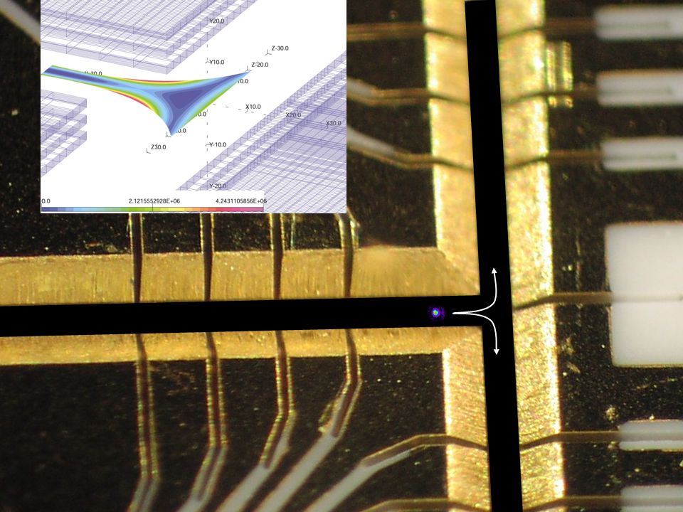
38. 1 mm “Tee” junction (Michigan)

41. 50 m

42. Microfabrication of Integral Trap structures (no assembly required) High aspect ratio Planar

43. Si doped GaAs AlGaAs Ge:Au ~10 mm GaAs Ion Trap Fabrication ~10 mm 100  m (Michigan)

44. Si doped GaAs AlGaAs Ge:Au ~10 mm 100  m GaAs Ion Trap Fabrication (Michigan)

45. Si doped GaAs AlGaAs Ge:Au ~10 mm 100  m GaAs Ion Trap Fabrication (Michigan)

46. Dan Stick Martin Madsen Winfried Hensinger Keith Schwab (LPS/UMd)

48. 6m6m

51. Progress… 2 m AlGaAs insulating gap: maximum voltage ~5V unable to load 4 m AlGaAs insulating gap: maximum voltage ~50 V (!) currently processing Other concerns… cantilever mechanical resonances  100 kHz RF dissipation P diss  V 0 2 C(R s C + tan) R s = series resistance C= electrode capacitance = rf drive frequency tan= loss tangent of insulating gap expect mW of dissipation for 50V trap operation e Q=CV RsRs C

52. Using a pho t on as the data bus: Entangling atoms and photons cavity-QED ENS-Paris CalTech MPQ-Garching … no direct measurement of entanglement: not enough control of either atom or photon

53. optical fiber trapped ions trapped ions Linking ideal quantum memory (trapped ion) with ideal quantum communication channel (photon)

54. 1,1 1,0 1,-1 0,0 2 S 1/2 2 P 3/2 F’=2 F’=1  2  (50 MHz)  10 8 /sec Probabalistic entanglement between a single atom and single photon   

55. 1,1 1,0 1,-1 0,0    (m=0)   (m=1) quant axis Given photon is emitted along quantization-axis: | = ||   + ||   (postselected)

56. PBS D1 D2 trapped ion collection lens polarization rotator |H  |V  excitation beam Schematic of Experiment microwaves measurement beam 1 m

57. Measured Correlations atom qubit photon qubit P(|H) = 97% P(|H) = 3% P(|V) = 6% P(|V) = 94%

58. Repeat, but rotate both qubits by =  /2 (relative phase ) before measurement. if initially in pure state |  = |  |V  + |  |H  then R|  = ( |  |V  + |  |H  ) cos(  + ( |  |H  + |  |V  ) sin(  correlation zero correlation |  |V  (p=50%) |  |H  (p=50%) |  |V  + |  |H  (p=50%) |  |H  + |  |V  (p=50%) if initially in 50-50 mixed state |  = then R|  =

59. Rotating each qubit By /2 before measurement: | | /2 /2 H V correlations in rotated basis P(|H) = 89% P(|H) = 11% P(|V) = 6% P(|V) = 94%

60. First direct observation of entanglement between a single atom and single photon. B. B. Blinov, et. al., Nature 428, 153 (2004) Entanglement Fidelity F=  ideal || ideal  > 87% Also: Bell Ineq. violation – D. Moehring et al., Phys. Rev. Lett. 93, 090410 (2004)

61. Can use this technique to seed remote ion-ion entanglement… Ann Arbor Columbus      V             V        1 2 D D coincidence photon detection upon coincidence photon detection        

62. Can use this technique to seed remote ion-ion entanglement… … and form the basis for scalable QC L.-M. Duan, et. al., Quantum Inf. Comp., 4, 165 (2004) quant-ph/0401020      V             V        1 2 D D coincidence photon detection upon coincidence photon detection         Ann Arbor Columbus

63. D D D D D D quantum repeater; distributed quantum computer

64. two ions in separate traps imaged on the same camera

65. Quantum Computer Physical Implementations 1. Individual atoms and photons a. ion traps b. atoms in optical lattices c. cavity-QED 2. Superconductors a. Cooper-pair boxes (charge qubits) b. rf-SQUIDS (flux qubits) 3. Semiconductors a. quantum dots b. phosphorus in silicon 4. Other condensed-matter a. electrons floating on liquid helium b. single phosphorus atoms in silicon scales works