1. Lecture 17 Nov 7, 2012 Discrete event simulation discrete time systems system changes with time, in discrete steps uncertainty (modeled by probability) interested in some aspect of outcome analytical vs. experimental approach to solution (latter is the “simulation” technique)

2. Discrete Event Simulation How to generate RV according to a specified distribution? binomial geometric Poisson etc. Examples of a Discrete Event System: traffic problem: given the locations of cars and destinations and traffic rules, what is the expected time for a specific car to reach its destination? repair problem: will be discussed in some detail and we will do a simulation using Matlab.

3. Outline What is discrete event simulation? Events Probability – review through examples Probability distributions Some examples

4. What is discrete event simulation? “ Simulation is the process of designing a model of a real system and conducting experiments with this model for the purpose either of understanding the behavior of the system or of evaluating various strategies (within the limits imposed by a criterion or set of criteria) for the operation of a system.” -Robert E Shannon 1975 “Simulation is the process of designing a dynamic model of an actual dynamic system for the purpose either of understanding the behavior of the system or of evaluating various strategies (within the limits imposed by a criterion or set of criteria) for the operation of a system.” -Ricki G Ingalls 2002 Definitions from http://staff.unak.is/not/andy/Year%203%2Simulation/Lectures/SIMLec2.pdf

5. What is discrete event simulation?  A simulation is a dynamic model that replicates the essential characteristics of a real system.  Simulations may be deterministic or stochastic, static or dynamic, continuous or discrete.  Discrete event simulation (DEVS) is stochastic, dynamic, and discrete.  DEVS is not necessarily spatial – it usually isn’t, but the ideas are applicable to many spatial simulations

6. What is discrete event simulation? DEVS has been around for decades, and is supported by a large set of supporting tools, programming languages (e.g. Simula, Simulink), conventional practices, etc. Like other kinds of simulation, offers an alternative, often simple way of solving a problem – simulate a system and observe results, instead of coming up with analytical model. Many other benefits like repeatability, ability to use multiple parameter sets, cheap compared to physical experiment, etc. (e.g. crash testing) Usually involves posing a question. The simulation estimates the answer.

7. What is discrete event simulation?  Stochastic (probabilistic) uncertainty is modeled as stochastic  Dynamic (changes over time)  Discrete (successive changes are separated by finite, usually, fixed amounts of time) Time may be modeled in a variety of ways within the simulation.

8. Alternate treatments of time Time divided into equal increments: Unequal increments: Cyclical: (e.g. traffic light or bus schedule)

9. Termination Simulation may terminate when a terminating condition is met. (e.g., when the queue is empty) May also be periodic. Can also be conceptually endless, like weather, terminated at some arbitrary time.

10. Random Variables A random variable (“X”) is numerical value associated with a random event. Ex 1: when rolling two dice, the sum of the values on the top faces) Ex 2: keep tossing a coin until you get a Head. The number of tosses could be the parameter of interest. In a stochastic Discrete Event System, the value associated with event is a random variable, that is its value has an associated probability. In Ex 2 above, the value is 2 with probability 0.25 By repeating the simulation, we can estimate the values of critical parameters.

11. Pseudorandom Number Generators A stochastic simulation depends on a pseudorandom number generator to generate usable random numbers. These generators can vary significantly in quality. For practical purposes, it may be important to check the random number generator you are using to make sure it behaves as expected. Using Matlab’s rand(), we can generate random real numbers between 0 and 1.

12. Exercise 1: Write a program that distributes a deck of 52 cards randomly to 4 people so that each one gets 13 cards. (e.g., hands of Bridge). Expected output format: >>[a,b,c,d] = shuffle(); >> a a = ‘A Hearts’ ‘2 Spades’ ‘8 Hearts’ …

13. Solution idea: More convenient to map cards to integers 1 to 52 so the problem is to divide 52 cards into four random piles of 13 each. If we can generate a vector v that represents a random permutation of 1:52, then, we can assign v(1:13) to a, etc. So the problem further reduces to: generate a random permutation of 1:52.

14. Two possible ideas 1)Start with v = 1:52, then randomly generate two integers j and k in the range 1:52, exchange v(j) and v(k) and repeat the process. Question: How many times should we do this before the deck is well shuffled? Tricky question to answer. 2)Start with v = 1:52 and randomly generate an integer j between 1 and 52 and exchange v(j) with v(52). Next generate an integer j between 1 and 51, and exchange v(j) with v(51) etc. We will next show that (2) works. You are to implement this.

15. Proof that (2) generates a random permutation of 1:52 Suppose a is the final permutation produced by the above algorithm. To show that (2) works, we need to show that the probability that any fixed permutation a = [i 1 i 2 … i 52 ] is generated by the above method is 1/52! We will not show this completely. But the main idea is the following. Prob( a(n) = i 52 ) is 1/52 since in the first step, all numbers from 1 to n have equal chance of being chosen, and thus i 52 has the same chance of 1/n. Similarly, we can see that Prob( a(n) = i 52 and a(n-1)= i 51 ) = 1/n(n-1) since in the second step, each of the remaining elements (other than i 52 ) has equal prob of 1/n-1 and the two events are independent. Extending this all the way to n steps, we conclude the claim.

16. Exercise 2: (coupon collector’s problem) When you buy a can of soda, it contains a coupon with a label in 1:n. The labels on the can are random in the sense that, at any point during simulation, the probability that the next can you buy will contain label j is 1/n. The goal is the determine the average number of cans you need to buy before you have collected all the n coupons.

17. Probability distributions In a Discrete Event Simulation, you need to decide what probability distribution functions best model the events. in most situations, uniform distribution does not work. Pseudorandom number generators generate numbers in a uniform distribution One basic trick is to transform that uniform distribution into other distributions. Some standard probability distributions are convenient to represent mathematically. They may or may not represent reality, but can be useful simplification.

18. Normal or Gaussian distribution  Ubiquitous in statistics  Many phenomena follow this distribution  When an experiment is repeated, the sum of the outcomes tend to be normally distributed.  We will demonstrate this experimentally using a Matlab simulation.

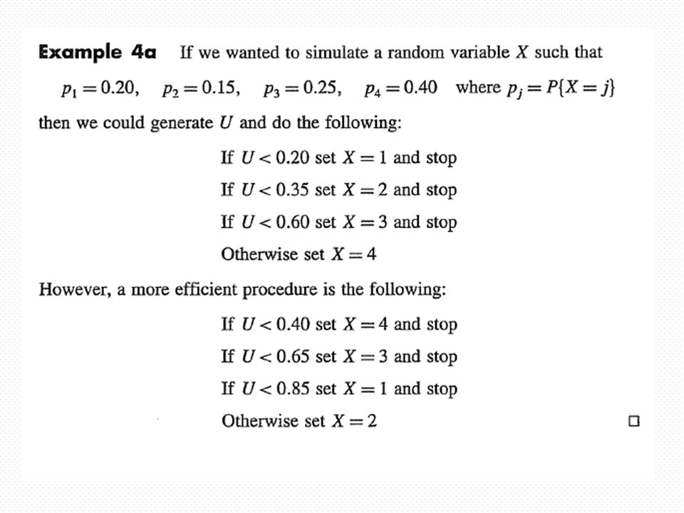
19. Simulating a Probability distribution Sampling values from an observational distribution with a given set of probabilities (“discrete inverse transform method”). Generate a random number U If U < p 0 return X 1 If U < p 0 + p 1 return X 2 If U < p 0 + p 1 + p 2 return X 3 etc. This can be speeded up by sorting p so that the larger intervals are processed first, reducing the number of steps.

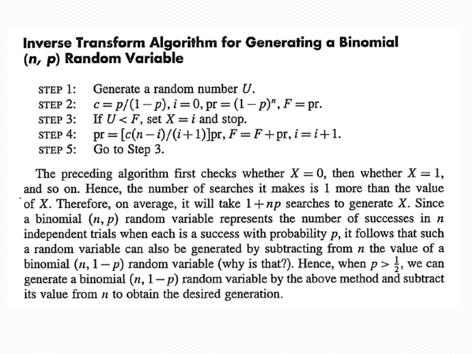
23. Poisson distribution Example of algorithm to sample from a distribution. X follows a Poisson distribution if: An algorithm for sampling from a Poisson distribution: 1. Generate a random number U 2. If i=0, p=e -l, F=p 3. If U < F, return I 4. P = l * p / (i + 1), F = F + p, i = i + 1 5. Go to 3 There are similar tricks to sampling from other probability distributions. Some of the distributions (e.g. Poisson, Normal etc.) can be generated using Matlab built in functions.

24. >>lambda = 2; >>random_sample1 = poissrnd(lambda,1,10) random_sample1 = 1 0 1 2 1 3 4 2 0 0 >>random_sample2 = poissrnd(lambda,[1 10]) random_sample2 = 1 1 1 5 0 3 2 2 3 4 >>random_sample3 = poissrnd(lambda(ones(1,10))) random_sample3 = 3 2 1 1 0 0 4 0 2 0 Poisson distribution – Matlab function

25. R = normrnd(mu,sigma,m,n,...) or R = normrnd(mu,sigma,[m,n,...]) generates an m-by-n-by-... array. The mu, sigma parameters can each be scalars or arrays of the same size as R. Examples n1 = normrnd(1:6,1./(1:6)) n1 = 2.1650 2.3134 3.0250 4.0879 4.8607 6.2827 n2 = normrnd(0,1,[1 5]) n2 = 0.0591 1.7971 0.2641 0.8717 -1.4462 n3 = normrnd([1 2 3;4 5 6],0.1,2,3) n3 = 0.9299 1.9361 2.9640 4.1246 5.0577 5.9864 Normal distribution – Matlab function

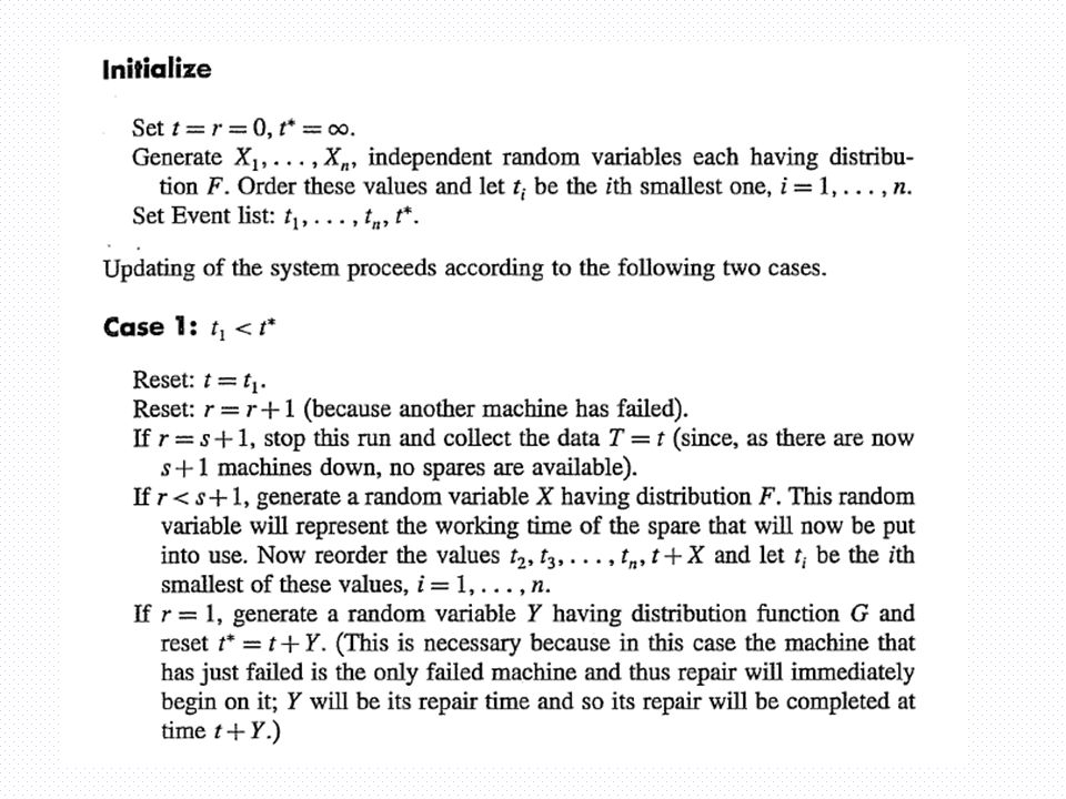
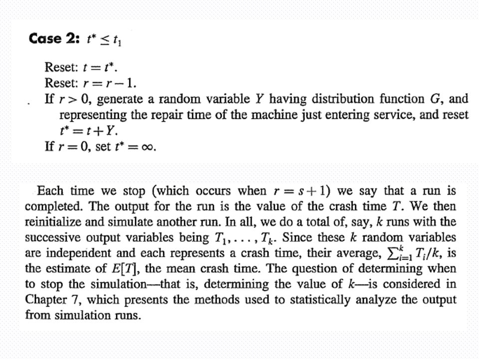
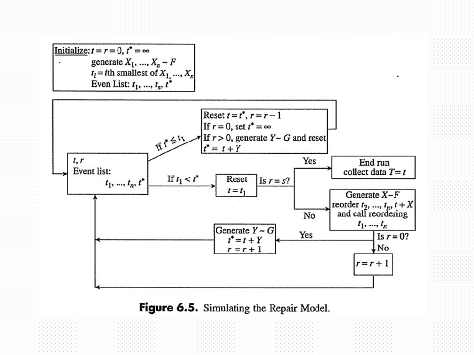
26. A repair problem n machines are needed to keep an operation. There are s spare machines. The machines in operation fail according to some known distribution (e.g. exponential, Poisson, uniform etc. with a known mean). When a machine fails, it is sent to repair shop and the time to fix is a random variable that follows a known distribution. Question: What is the expected time for the system to crash? System crashes when fewer than n machines are available.

27. n = number of working machines needed S = number of spares available

32. Matlab implementation