1. Zac Adelman and Craig Mattocks Carolina Environmental Program
Air Quality Modeling
∂C/ ∂t = - ∂(uC)/ ∂x - ∂(vC)/ ∂y - ∂(wC)/ ∂z
J = ∫ 4πIλ,T Aλ,T QYλ,T dλ ∞
kr = Ar(300/T)Bexp(Cr/T)
dx = (Recosφ)dλe
Zac Adelman and Craig Mattocks Carolina Environmental Program

2. Outline Why model air pollution?
Air quality modeling system components
Meteorology
Emissions
Chemistry and transport
Technical and operational details
Problems in air quality modeling
Application examples
Future directions in atmospheric modeling

3. SO2 (g) SO2 (aq) O3 + NO  NO2 + O2 O + O2 + M  O3 + M Source Sink
Aqueous Chemistry:
SO2 (g) SO2 (aq)
O3 + NO  NO2 + O2
O + O2 + M  O3 + M
Gas Chemistry:
Aerosol Processes:
Condensation & Deposition
Evaporation & Sublimation
Nucleation & Coagulation
Advection Diffusion
Boundary Conditions
Biogenic Emissions
Anthropogenic Emissions
Geogenic Emissions
Adapted from Mackenzie and Mackenzie, “Our Changing Planet”, Prentice Hall, New Jersey, 1995.
Source
Sink

4. Why model air pollution?
Air pollution models are frameworks that integrate our understanding of individual processes with atmospheric measurements
Air pollution systems are non-linear
Need to establish the link between emissions sources and ambient concentrations

5. Air Quality Modeling Components
Meteorology modeling
Emissions processing
Initial/boundary conditions processing
Photolysis rate processing
Chemistry and transport modeling

6. WRF-ARW Basics Fundamentals of Numerical Weather Prediction
Real vs. artificial atmosphere
Map projections
Horizontal grid staggering
Vertical coordinate systems
Definitions & Acronyms
Flavors of WRF
ARW core
NMM core
Other Numerical Weather Prediction Models
MM5
ARPS
Global Icosahedral
WRF Model Governing Equations
Vertical coordinate and grid discretization
Time integration
Microphysics
Current Defects of WRF

7. Real vs. Artificial Atmosphere
True analytical solutions are unknown!
Numerical models are discrete approximations of a continuous fluid.

8. Map Projections x = r cos  y = r 
Example of a regional high resolution grid (projection of a spherical surface onto a 2D plane) nested within a global (lat,lon) grid with spherical coordinates
x = r cos  y = r 
Differences in map projections require caution when dealing with flow of information across grid boundaries.
WRF offers polar stereographic, Lambert conformal, Mercator and rotated Lat-Lon map projections.

9. Arakawa “A” Grid Unstaggered grid - all variables defined everywhere.
Poor performance, first grid geometry employed in NWP models.
Noisy - large errors, short waves propagate energy in wrong direction, additional smoothing required.
Poorest at geostrophic adjustment - wave energy trapped, heights remain too high.
Can use a 2x larger time step than staggered grids.

10. Arakawa “B” Grid Staggered, velocity at corners.
Preferred at coarse resolution.
Superior for poorly resolved inertia-gravity waves.
Good for geostrophy, Rossby waves: collocation of velocity points.
Bad for gravity waves: computational checkerboard mode.
Used by MM5 model.

11. Arakawa “C” Grid
Staggered, mass at center, normal velocity, fluxes at grid cell faces, vorticity at corners.
Preferred at fine resolution.
Superior for gravity waves.
Good for well resolved inertia-gravity waves.
Simulates Kelvin waves (shoulder on boundary) well.
Bad for poorly resolved waves: Rossby waves (computational checkerboard mode) and inertia-gravity waves due to averaging the Coriolis force.
Used by WRF-ARW, ARPS, CMAQ models.

12. Arakawa “D” Grid
Staggered, mass at center, tangential velocity along grid faces.
Poorest performance, worst dispersion properties, rarely used.
Noisy - large errors, short waves propagate energy in wrong direction.

13. Arakawa “E” Grid Semi-staggered grid.
Equivalent to superposition of 2 C-grids, then rotated 45 degrees.
Center set to translated (lat,lon) = (0,0) to prevent distortion near edges, poles.
Developed for Eta step-mountain coordinate to enhance blocking, overcome PGF errors caused by sigma coordinates.
Controls the cascade of energy toward smaller scales.
Used by WRF-NMM and Eta models.

17. Definitions & Acronyms
WRF: Weather Research & Forecasting numerical weather prediction model
ARW: Advanced Research WRF [nee Eulerian Model (EM)] core
NMM: Nonhydrostatic Mesoscale Model core
WRF-SI: Standard Initialization (4 components) - prepares real atmospheric data for input to WRF
WRF-VAR: Variational 3D/4D data assimilation system (not used for this class)
IDV: Integrated Data Viewer - Java application for interactive visualization of WRF model output

18. Flavors of WRF (ARW) ARW solver (research - NCAR, Boulder, Colorado)
Fully compressible, nonhydrostatic equations with hydrostatic option
Arakawa-C horizontal grid staggering
Mass-based terrain following vertical coordinate
Vertical grid spacing can vary with height
Top is a constant pressure surface
Scalar-conserving flux form for prognostic model variables
2nd to 6th-order advection options in horizontal &vertical
One-way, two-way and movable nest options
Runge-Kutta 2nd & 3rd-order time integration options
Time-splitting
Large time step for advection
Small time step for acoustic and internal gravity waves
Small step horizontally explicit, vertically implicit
Divergence damping for suppressing sound waves
Full physics options for land surface, PBL, radiation, microphysics and cumulus parameterization
WRF-chem under development:

19. Flavors of WRF (NMM)
NMM solver (operational - NCEP, Camp Springs, Maryland)
Fully compressible, nonhydrostatic equations with reduced hydrostatic option
Arakawa-E horizontal grid staggering, rotated latitude-longitude
Hybrid sigma-pressure vertical coordinate
Conservative, positive definite, flux-corrected scheme used for horizontal and vertical advection of TKE and water species
2nd-order spatial that conserves a number of 1st-order and quadratic quantities, including energy and enstrophy
One-way, two-way and movable nesting options
Time-integration schemes: forward-backward for horizontally propagating fast waves, implicit for vertically propagating sound waves, Adams-Bashforth for horizontal advection and Coriolis force, and Crank-Nicholson for vertical advection
Divergence damping & E subgrid coupling for suppressing sound waves
Full physics options for land surface, PBL, radiation, microphysics (only Ferrier scheme) and cumulus parameterization
Note: Many ARW core options are not yet implemented! Nesting still under development
NMM core will be used for HWRF (hurricane version of WRF), operational in summer of 2007

20. Other NWP Models (MM5) MM5 (research - PSU/NCAR, Boulder, Colorado)
Progenitor of WRF-ARW, mature NWP model with extensive configuration options
Support terminated, no future enhancements by NCAR’s MMM division
Nonhydrostatic and hydrostatic frameworks
Arakawa-B horizontal grid staggering
Terrain following sigma vertical coordinate
Unsophisticated advective transport schemes cause dispersion, dissipation, poor mass conservation, lack of shape preservation
Outdated Leapfrog time integration scheme
One-way and two-way (including movable) nesting options
4-dimensional data assimilation via nudging (Newtonian relaxation), 3D-VAR, and adjoint model
Full physics options for land surface, PBL, radiation, microphysics and cumulus parameterization

21. Other NWP Models (ARPS)
ARPS (research - CAPS/OU, Norman, Oklahoma)
Advanced Regional Prediction System
Sophisticated NWP model with capabilities similar to WRF
Primarily used for tornado simulations at ultra-high (25 meter) resolutions and assimilation of experimental radar data at mesoscale
Elegant, source code, easy to read/understand/modify, ideal for research projects, very helpful scientists at CAPS
Arakawa-C horizontal grid staggering
Currently lacks full mass conservation and Runge-Kutta time integration scheme
ARPS Data Assimilation System (ADAS) under active development/enhancement (MPI version soon), faster & more flexible than WRF-SI, employed in LEAD NSF cyber-infrastructure project
wrf2arps and arps2wrf data set conversion programs available

22. Global Icosahedral Model

23. WRF Model Governing Equations (Eulerian Flux Form)
Momentum:
∂U/∂t + (∇ · Vu) − ∂(pφη)/∂x + ∂(pφx)/∂η = FU
∂V/∂t + (∇ · Vv) − ∂(pφη)/∂y + ∂(pφy)/∂η = FV
∂W/∂t + (∇ · Vw) − g(∂p/∂η − μ) = FW
Potential Temperature:
Diagnostic Hydrostatic (inverse density a):
∂Θ/∂t + (∇ · Vθ) = FΘ
∂φ/∂η = -μ
Continuity:
where:
μ = column mass
V = μv = (U,V,W)
Ω = μ d(η)/dt
Θ = μθ
∂μ/∂t + (∇ · V) = 0
Geopotential Height:
∂φ/∂t + μ−1[(V · ∇φ) − gW] = 0

24. WRF Vertical Coordinate h

25. Vertical Grid Discretization

26. Runge-Kutta Time Integration
Φ∗ = Φt + t/3 R(Φt )
Φ∗∗ = Φt + t/2 R(Φ∗)
Φt+t = Φt + t R(Φ∗∗)
“2.5” Order Scheme
Linear: rd order
Non-linear: 2nd order
Square Wave Advection Tests:

27. Runge-Kutta Time Step Constraint
RK3 is limited by the advective Courant number (ut/x) and the user’s choice of advection schemes (2nd through 6th order)
The maximum stable Courant numbers for advection in the RK3 scheme are almost double those in the leapfrog time-integration scheme
Maximum Courant number for 1D advection in RK3
Time Scheme
Spatial order
3rd
4th
5th
6th
Leapfrog
Unstable
0.72
0.62
RK2
0.88
0.30
RK3
1.61
1.26
1.42
1.08

28. Microphysics
Includes explicitly resolved water vapor, cloud and precipitation processes
Model accommodates any number of mixing-ratio variables
Four-dimensional arrays with 3 spatial indices and one species index
Memory (size of 4th dimension) is allocated depending on the scheme
Carried out at the end of the time-step as an adjustment process, does not provide tendencies
Rationale: condensation adjustment should be at the end of the time step to guarantee that the final saturation balance is accurate for the updated temperature and moisture
Latent heating forcing for potential temperature during dynamical sub-steps (saving the microphysical heating as an approximation for the next time step)
Sedimentation process is accounted for, a smaller time step is allowed to calculate vertical flux of precipitation to prevent instability
Saturation adjustment is also included

29. WRF Microphysics Options
Mixed-phase processes are those that result from the interaction of ice and water particles (e.g. riming that produces graupel or hail)
For grid sizes ≤ 10 km, where updrafts may be resolved, mixed-phase schemes should be used, particularly in convective or icing situations
For coarser grids the added expense of these schemes is not worth it because riming is not likely to be resolved
Scheme
Number of Moisture Variables
Ice-Phase Processes
Mixed-Phase Processes
Kessler 3 N
Purdue Lin 6 Y
WSM3
WSM5 5
WSM6
Eta GCP 2
Thompson 7

30. Current Defects of WRF
Serious deficiencies in PBL parameterizations and land surface models produce biases/errors in the predicted surface and 2-meter temperatures, and PBL height. WRF cannot maintain shallow stable layers.
3D/4D Variational data assimilation and Ensemble Kalman Filtering (EnKF) still under development, EnKF available to community from NCAR as part of the Data Assimilation Research Testbed (DART).
Not clear yet what to do in “convective no-man’s land” – convective parameterizations valid only at horizontal scales > 10 km, but needed to trigger convection at 5-10 km scales.
Multi-species microphysics schemes with more accurate particle size distributions and multiple moments should be developed to rectify errors in the prediction of convective cells.
Heat and momentum exchange coefficients need to be improved for high-wind conditions in order to forecast hurricane intensity. Wind wave and sea spray coupling should also be implemented. Movable, vortex-following 2-way interactive nested grid capability has recently been incorporated into the WRF framework.
Upper atmospheric processes (gravity wave drag and stratospheric physics) need to be improved for coupling with global models.

31. Emissions Processing Emissions Processing Steps Area Mobile Point
Biogenic
Emissions Processing Steps
AQM-ready Emissions:

32. Emissions Terminology
Inventory: estimate of pollutant emissions at a given spatial unit
Model Grid: 3-d representation of the earths surface based on discrete and uniform spatial units, i.e. grid cells
Speciation: conversion of inventory pollutant species to model pollutant species
Gridding: conversion of inventory spatial units to model grid cells
Temporalization: conversion of inventory temporal units to those requires by an air quality model

33. Emissions Terminology
Plume rise: calculation of the vertical distribution of emissions from point sources and the subsequent allocation of the emissions to the model layers
Spatial surrogate: GIS-based estimate of the fraction of a grid cell covered by a particular land-use category (e.g. population or rural housing)
Profiles: emissions distributions in space, time, or to chemical species
Cross-referencing: relating profiles to specific emissions sources

34. Area sources Most basic inventory unit
Country/province/municipality wide estimate
Requires spatial surrogates to map to a model grid
Examples
Construction and agricultural emissions
Road dust
Fires

35. Mobile sources On-road: Estimate by road way and vehicle type
Requires emissions factors for local vehicles and activities/speeds for local roads
Gridding by road way distribution or links
Can use local meteorology to adjust emissions factors for temperature and humidity
Examples: Heavy-duty diesel trucks on primary highways, light-duty gasoline cars on rural roads
Non-road: Area-like estimates
Examples: Construction and mining vehicles, recreational vehicles (boats, ATV’s),

36. Point sources Emissions at specific latitude-longitude coordinates
Often elevated sources that require stack parameters (e.g. stack height, exit gas velocities, exit gas temperatures, etc.)
Can use annual, daily, or hourly emissions estimates
Examples:
Electricity generating units (EGU’s)
Smelters
Wildfires

37. Biogenic sources Estimates of emissions from vegetation and soils
Uses gridded land-use data and emissions factors by vegetation type
Uses local meteorology to calculate emissions based on photosynthetically active radiation (PAR) and to adjust for temperatures
Examples:
VOC emissions from specific tree species
Soil NO

38. Gridded sources Pre-gridded emissions from global databases
Normalize to the model grid to combine with other sources
Can encompass any of the emissions categories
Top-down vs. bottom-up emissions estimate

39. Emissions Processing
Purpose: convert emissions data to formats required by air quality model
Primary functions
Import data into system
Spatial allocation (gridding)
Chemical allocation (speciation)
Temporal allocation
Merge
Quality assurance

40. Emissions Processing Steps
Data Import
Inventory categories
Area
Point
Mobile
Biogenic
Gridded
ASCII or gridded binary
Country/state/county estimates
Annual estimates
Pollutants include bulk VOC and PM2.5
Spatial Allocation
Inventory spatial units  model grid
Requires spatial surrogates
EI  Grid Cell Mapping

41. Emissions Processing Steps
Chemical Allocation
Tons  Moles
Converts inventory pollutants to air quality model species
Model-dependent speciation profiles
NOx  NO + NO2
VOC  PAR, OLE, etc.
PM2.5  NO3, SO4, etc.
Temporal allocation
Inventory units  hourly emissions
Requires temporal profiles
Monthly
Weekly
Diurnal

42. Emissions Processing Steps
Merging
Combine all intermediate steps to create AQM-ready emissions
Combine individual source categories
Formatting
Units
Output file naming
Quality Assurance
Report base inventory values and changes at each processing step
Customize reporting
e.g. by state and SCC, by SCC and temporal profiles, by grid cell and surrogate I.D.
Means to determine why a result occurred

43. Other Emissions Processing Steps
Plume Rise
Allocate elevated emissions sources to vertical model layers
Compute layer fractions
Require meteorology to calculate plume buoyancy
Stationary point, fires, in-flight aircraft
Projections
Grow and/or control inventories for future year modeling
Source-based projection information

44. Emissions Processing Paradigms
Linear
Sequential steps that follow a particular order
Requires completing one step before completing the next
Parallel
Flexible sequence with steps in any order
Import
Grid
Speciate
Temporal
Merge
AQM
Import
Grid
Speciate
Temporal
Merge
AQM

45. Initial and Boundary Conditions
Initial conditions define the chemical conditions at the start of a simulation
Defined using vertical profiles of clean background concentrations
Boundary conditions define the chemical conditions on the horizontal faces of the modeling domain
Static and dynamic boundaries are possible
Initial conditions decay exponentially with simulation time; boundary conditions on the upwind boundary continue to affect predictions through an entire simulation.

46. Initial/Boundary Condition Processing
Processing requires generating IC/BC estimates on a model-grid
Nested simulations extract BC’s from a parent grid
Multi-day simulations extract IC’s from the last hour of the previous day

47. Photolysis Rate Processing
Photolysis: Chemical dissociation caused by the absorption of solar radiation
Photolysis rate: rate of reaction for pollutants that undergo photolysis
Processing calculates clear sky photolysis rates at different latitudes and altitudes
Air quality models adjust rates with cloud cover estimates from meteorology
J = ∫ 4πIλ,T Aλ,T QYλ,T dλ ∞

48. What are air quality models?
Statistical models: describe concentrations in the future as a statistical function of current chemical and/or meteorological conditions
Chemistry-transport models (CTM): based on fundamental descriptions of physical and chemical processes in the atmosphere

49. How do CTMs work? Air Quality Model processes
Dynamical/thermodynamical: meteorology, land surface conditions (soil, water)
Transport: emissions, advection, diffusion, dry deposition, sedimentation
Gas phase chemistry: photochemistry, phase changes
Radiative: optical depth, visibility, energy transfer
Aerosol/clouds: nucleation, coagulation, heterogeneous chemistry, aqueous chemistry

50. Overlay 3-D boxes on a grid
Lagrangian/Trajectory Models
Moves relative to the coordinate
Different locations at different times
Only emissions enter the cell
No material leaves the cell

51. Overlay 3-D boxes on a grid
Eulerian Models
Fixed relative to the coordinate
All locations at all times
Materials move through all cell faces*

52. Conceptual approach to CTMs
Extend the 2-D box model to three dimensions
2-D
3-D ∆x ∆x ∆z
u1C1
u2C2
u2C2
u1C1 Ci ∆y Ci ∆y
Basic Continuity Equation (flux in 1 direction):
∆C ∆x ∆y ∆z = u1C1∆y ∆z ∆t – u2C2 ∆y ∆z ∆t
Divide by ∆t and volume: ∂C/ ∂t = - ∂(uC)/ ∂x
u = wind vector
Ci = concentration of species i

53. Expanded Continuity Equation
w2C2
3-D ∆x ∆z
u2C2
u1C1
Expanded Continuity Equation Derivation:
Expand to flux three dimensions:
∂C/ ∂t = - ∂(uC)/ ∂x - ∂(vC)/ ∂y - ∂(wC)/ ∂z
= ∙ (vC) (flux divergence form)
Add additional production and loss terms:
∂C/ ∂t + ∙ (vC) = D 2 C + R + E - S Ri X
v1C1 ∆y E S
w1C1
u,v,w = wind vectors
E = emissions
S = loss processes
Ri = Chemical formation of species I
D = Molecular diffusion coefficient

54. Rnuc + Rc/e + Rdp/s + Rds/e + Rhr
Aqueous Chemistry:
Gas Chemistry:
Aerosol Processes:
Rchem
Rhr
Rnuc + Rc/e + Rdp/s + Rds/e + Rhr
Diffusion: D C
Advection: ∙ (vC)
Boundary Conditions
Remis
Rdep
Rwash
R = Rate
chem=chemical production/loss hr=heterogeneous reactions nuc=nucleation c/ev=condensation/evaporation dp/s=depositional growth/sublimation ds/e=dissolution/evaporation wash=washout dep=deposition emis=emissions

55. Full Continuity Equations
Gas Continuity Equation
∂C/ ∂t + ∙ (vC) = D 2 C + Rchemg + Remisg + Rdepg+ Rwashg + Rnucg + Rc/eg + Rdp/sg + Rds/eg + Rhrg
Particle Continuity Equation (number)
∂n/ ∂t + ∙ (vn) = D 2 n + Remisn + Rdepn+ Rsedn + Rnucn
+ Rwashn + Rcoagn
Particle Continuity Equation (volume concentration)
∂V/ ∂t + ∙ (vV) = D 2 V + Remisv + Rdepv+ Rsedv + Rnucv
+ Rwashv + Rcoagv+ Rc/ev + Rdp/sv + Rds/ev
+ Regv + Rqgv + Rhrv

56. CTM Coordinate Systems
Convert all motion equations from Cartesian to spherical coordinates
Horizontal grids typically on the order of 1 to 36 km
Recent applications extending to 500m and 108 km
Lambert conformal, polar stereographic, and Mercator are the most common modeling projections
dx = (Recosφ)dλe dy = Red φ

57. CTM Coordinate Systems
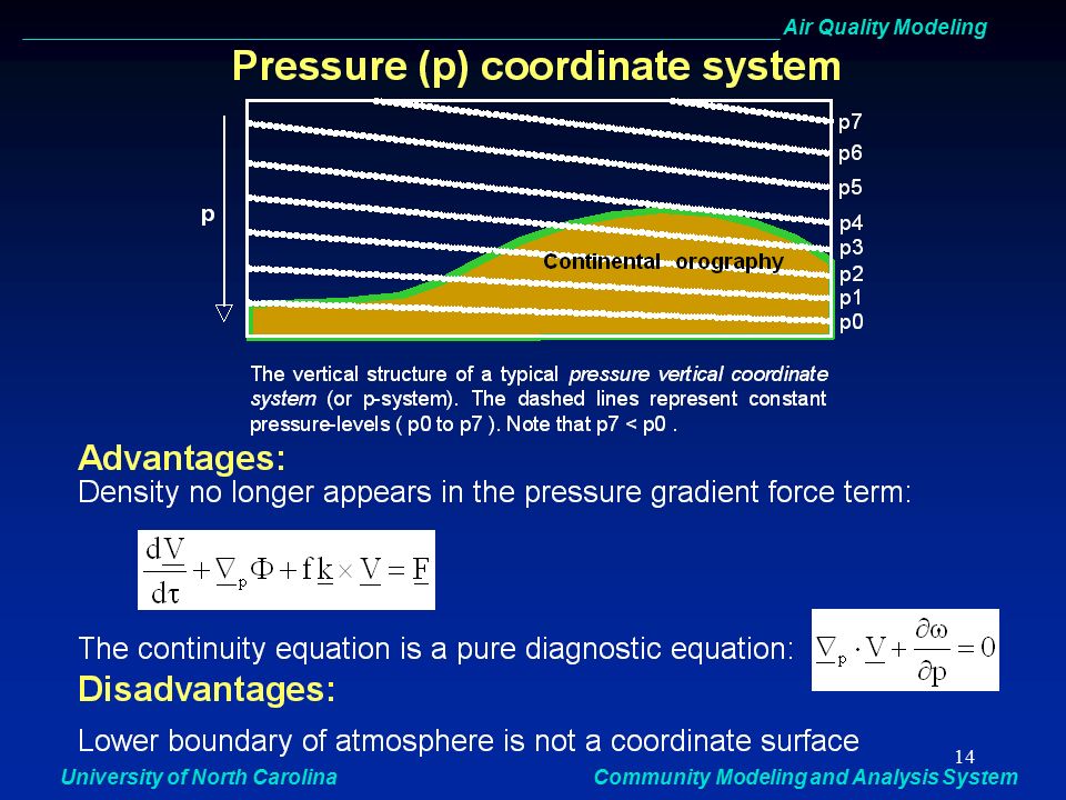
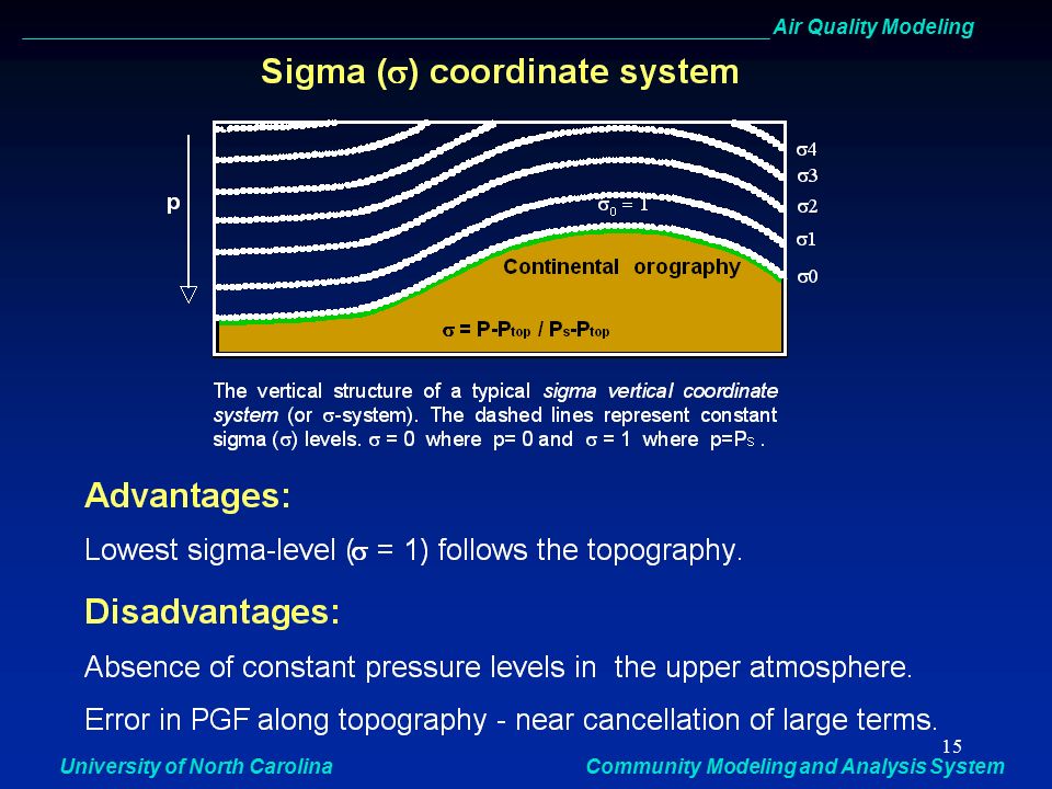
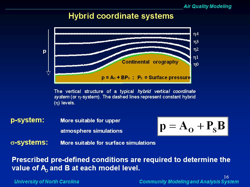
Vertical grids extend from the surface to 10 km
Altitude coordinate: layers are defined as surfaces of constant height with variable pressure
Pressure coordinate: layers are defined as surfaces of constant pressure with variable height
Sigma-pressure coordinate: layers defined as surfaces of constant σ, where
pa – pa,top
pa, surf - pa,top
σ =
(0,1)

58. Boundary Layer Processes
Boundary layer more difficult to model because of greater turbulence and larger emissions forcing terms than in free troposphere; land surface interactions and planetary boundary layer (PBL) dynamics dominate
Surface temperature and soil moisture affect energy and moisture flux; affect mixing heights, winds, and pollutant concentrations

59. Modeled cloud processes
Aerosol particle
Radiative transfer: reflecting, scattering, and trapping heat
Atmospheric component of the hydrologic cycle
Wet deposition of gases and particles
Medium for aqueous phase chemistry
Vertical transport/convective mixing
Energy balance: temperature effects and photolysis rates
Aerosol Processes
Condensation
Gas Phase
Water Droplet
pA pA(a) A(a) A(r)
B(a) B(r)
pC pC(a) C(a) C(r)
Evaporation
New aerosol particle

60. Energy/Radiative Effects
Visibility
Optical depth
scattering and absorption between top of atmosphere and altitude x
Photolysis rates
dI/dx = σ bIB - σ ext I
σ = extinction coefficient
I = visible radiance
Radiative transfer
Sun
Beam
(μ,Θ)
Fs (-μ,Θ) Θ
Multiple scattering
Direct
J = ∫ 4πIλ,T Aλ,T QYλ,T dλ ∞
Single scattering Θs
Diffuse
4πI = actinic flux A = absorption cross section QY = quantum yield

61. Gas Phase Chemistry Carbon bond lumping Molecular lumping
Thousands of different organic and inorganic gases react to form smog and PM
Gas phase chemistry is a “stiff” system
Parameterized chemistry mechanisms represent the system with a few surrogate organic pollutants
Surrogates based on molecular or atomic structures of pollutants
Carbon bond lumping
Propane = 3 PAR:
H3C-CH2-CH3
1-Butene = 2 PAR + 1 OLE:
H2C=CH-CH3-CH3
averaged reaction rates
Molecular lumping
Surrogates represent similarly reactive species
Explicit or averaged reaction rates

62. Gas Phase Chemistry Important Organic Reactions (methane example)
OH + CH4  H2O + CH3∙
CH3∙ + O2  CH3O2∙
CH3O2∙ + NO  NO2 + CH3O∙
CH3O∙ + O2  HO2 + HCHO
CH3O2∙ + HO2  O2 + CH3O2H
CH3O2H + hv  CH3O∙ (λ<360 nm)
CH3O2H + OH  H2O + CH3O2∙
Important Inorganic Reactions
NO + O3  NO2 + O2
NO2 + hv  NO + O (λ<420 nm)
O + O2 + M  O3 + M
O3 + hv  O2 + O(1D) (λ<310 nm)
O3 + hv  O2 + O3P (λ>310 nm)
O(1D) + H2O  2OH
OH + O3  HO2 + O2
OH + NO  HONO
HONO + hv  OH + NO (λ<400 nm)
NO2 + OH  HNO3
HNO3 + hv  NO2 + OH (λ<335 nm)

63. Gas Phase Chemistry Key reaction sequence for smog
ROG∙ + NO  NO2 + ROG∙∙
NO + O3  NO2 + O2
NO2 + hv  NO + O
O + O2 + M  O3 + M

64. Gas Phase Chemistry Kinetics J = ∫ 4πIλ,T Aλ,T QYλ,T dλ
aA + bB  eE + fF Rate = kr[A]a[B]b
Rate constant calculations
d[A]t/dt = -kF[A]t = -kS[A]t[B]0 = -kT[A]t[B]0[C]0
1st order: A  D + E kF = -(1/t) ln [A]t/[A]0
2nd order: A + B  D + E kS = -(1/[B]0t) ln [A]t/[A]0
3rd order: A + B + C  D + E kT = -(1/[B]0[C]0t) ln [A]t/[A]0
Arrhenius equation for temperature dependence
kr = Ar(300/T)Bexp(Cr/T)
Troe equation for temperature and pressure dependence
kr = {(k∞,T k0,T [M])/(k∞,T+k0,T[M])}Fc [1+(logk0[M]/k∞)^2]^-1
Photolysis rate equation
J = ∫ 4πIλ,T Aλ,T QYλ,T dλ ∞

65. Aqueous Chemistry
Gases equilibrate with the aqueous phase by Henry’s law:
[A(aq)] = HApA
Dissolved gases react in solution to form new compounds
Sequence: droplet formation  gases dissolve in droplet  chemical reactions  evaporation

66. Aerosol Dynamics
Size distribution: ratio of # aerosols in a diameter range to the size of the range; discrete function of the number of particles
Ni = ni∆Dp
Number distribution: continuous function of the diameter of the particles
N = ∫ nN(Dp)dDp
Aerosol moments: properties of the distributions (e.g. mean, variance) ∞

67. Aerosol Dynamics
Mass transfer solutions to transport mass between gas/aqueous/solid phases
Solve gravitational settling, diffusion, and advection for moving particles around
4 classes of nucleation for particle formation:
Homogenous  Homomolecular
Homogenous  Heteromolecular
Heterogenous  Homomolecular
Heterogenous  Heteromolecular

68. CTM Setup and Configuration
All CTM’s are free and open source
Compile on UNIX/Linux with Fortran
Script interfaces for compiling and running
Begin with download, installation, and compilation
Set up computing environment
I/O directories
Check for processor availability and disk space

69. CTM Setup and Configuration
CTM’s are at the end of a long sequence of preprocessing steps
Prepare meteorology inputs with research and forecast met models
Prepare emissions inputs with specialized emissions processors
Prepare initial and boundary condition inputs with preprocessors packaged with CTM
Generate clear sky photolysis rates with a preprocessor packaged with CTM

70. CTM Process Schematic Hourly Concentrations Model Ready Emissions
Met
Modeling
Emissions IC
Preparation BC
Photolysis
Rates
2-D/3-D Met
Files
Model Ready
Input File
Clear Sky
J Rates
CTM
Hourly
Concentrations
Cumulative
Wet Dep
Dry Dep
Visibility Metrics
Diagnostic
Outputs

71. Modeling Conventions Establish base case model performance
Simulate sensitivities off the base case
Select episodes or time periods that illustrate the problem being addressed
O3 episodes
PM episodes
High flow regimes/transport scenarios
Annual episodes for one-atmosphere modeling

72. One Atmosphere Approach
Changing paradigm from multiple models that address individual process to a single unified model
Conceptually more realistic: all atmospheric processes are coupled
In practice very difficult because of confounding errors
“Right answer for the wrong reasons”

73. What is the right answer for CTMs?
Evaluation techniques
Comparisons to ambient measurements
Sanity checks
Looking for known trends (diurnal/seasonal patterns, chemical signatures (ratios)
Comparison to measurements
Paired in space and time
Compare predicted vs observed maximums
Paired in space but not in time
Statistical metrics include paired/unpaired peak prediction accuracy, mean normalized bias, mean error

74. Problems in air quality modeling
Inconsistencies in spatial scales and speciation when comparing models to measurements
Incomplete measurement database (PBL, radiation budget, short lived pollutants, observations aloft)
Huge uncertainties in all input data
Garbage in = Garbage out

75. Problems in air quality modeling
Met and chemistry models are tuned for certain conditions
Meteorology models generally don’t work well under stagnant, low flow conditions
Chemistry models break down at night and during background ambient conditions
Incomplete science
For various reasons, some important atmospheric processes are either not represented at all or are using crude approximations

76. Significant CTM Studies
Regional Ozone Model: early 1980’s, first regional scale model, early studies on regional transport
Regional Acid Deposition Model: mid 1980’s, 1st multi-pollutant model, predecessor to current modeling systems
National Acid Precipitation Assessment (NAPAP): 1980’s, established links between S emissions in the Midwest to acid rain in the Northeast; first modeling studies of emissions trading programs

77. Significant CTM Studies
Ozone Transport Assessment Group (OTAG): mid 1990’s, established multi-scale problem of ozone, relationships between 1-hr vs. 8-hr ozone standard and transport, prevailing regional conditions for poor air quality, weekday-weekend trends in air quality

78. Model Application Examples
Regional Ozone Sensitivities - NCDAQ
Combined Area, Mobile, Point Reductions
Base June, 1996
Combined Area, Mobile, Point Reductions
Across the board Area, Mobile Reductions

79. Model Application Examples
Intercontinental transport of pollutants

80. Model Application Examples
Continental one atmosphere modeling
1 day, 24-hour average ozone
Observations overlaid on plot

81. Model Application Examples
Continental one atmosphere modeling
Summer, 2002 Sulfate
Winter, 2002 Nitrate

82. Future Directions Quantify model uncertainties
Expand the ability of the models to represent and integrate all atmospheric processes
2-way coupling between global, regional, and neighborhood scale models
Source apportionment technologies
Couple with other media/disciplines (water,soil,risk, economics)
Community/open source development