Applied Quantitative Methods MBA course Montenegro

Applied Quantitative Methods MBA course Montenegro
Peter Balogh PhD

Statistical inference

Introduction So far, most of this book has been about describing situations. This is useful and helps in communication, but would not justify doing a whole book or course. In this part we are going to the next step and looking at ways of extending or generalizing our results so that they not only apply to the group of people or set of objects which we have measured, but also to the whole population. As we saw in Part 1, most of the time we are only actually examining a sample, and not the whole population. Although we will take as much care as possible to ensure that this sample is representative of the population, there may be times when it cannot represent everything about the whole group. The exact results which we get from a sample will depend on chance, since the actual individuals chosen to take part in a survey may well be chosen by random sampling (where every person has a particular probability of being selected).

Introduction We need to distinguish between values obtained from a sample, and thus subject to chance, and those calculated from the whole population, which will not be subject to this effect. We will need to also distinguish between those true population values that we have calculated, and those that we can estimate from our sample results. Some samples may be 'better' than others and we need some method of determining this. Some problems may need results that we can be very sure about, others may just want a general idea of which direction things are moving. We need to begin to say how good our results are.

Introduction Sample values are no more than estimates of the true population values (or parameters or population parameters). To know these values with certainty, your sample would have to be 100%, or a census. In practice, we use samples that are only a tiny fraction of the population for reasons of cost, time and because they are adequate for the purpose. How close the estimates are to the population parameters will depend upon the size of the sample, the sample design (e.g. stratification can improve the representativeness of the sample), and the variability in the population. It is also necessary to decide how certain we want to be about the results; if, for example, we want a very small margin of sampling error, then we will need to incur the cost of a larger sample design. The relationship between sample size, variability of the population and the degree of confidence required in the results is the key to understanding the chapters in this part of the book.

Introduction The approach in Chapter 13 is different, as it is concerned with data that cannot easily or effectively be described by parameters (e.g. the mean and standard deviation). If we are interested in characteristics (e.g. smoking/non-smoking), ranking (e.g. ranking chocolate products in terms of appearance) or scoring (e.g. giving a score between 1 and 5 to describe whether you agree or disagree with a certain statement), a number of tests have been developed that do not require description by the use of parameters. After working through these chapters you should be able to say how good your data is, and test propositions in a variety of ways.

Inference quick start Inference is about generalizing your sample results to the whole population. The basic elements of inference are: confidence intervals parametric significance tests non-parametric significance tests. The aim is to reduce the time and cost of data collection while enabling us to generalize the results to the whole population. It allows us to place a level of confidence on our results which indicates how sure we are of the assertions we are making. Results follow from the central limit theorem and the characteristics of the Normal distribution for parametric tests.

Inference quick start Key relationships are:
Ninety-five percent confidence interval for a mean: Ninety-five percent confidence interval for a percentage:

Inference quick start Where there is no cardinal data, then we can use non-parametric tests such as chi-squared.

11. Confidence intervals This chapter allows us to begin to answer the question: 'What can we do with the sample results we obtain, and how do we relate them to the original population?' Sampling, as we have seen in Chapter 3, is concerned with the collection of data from a (usually small) group selected from a defined, relevant population. Various methods are used to select the sample from this population, the main distinction being between those methods based on random sampling and those which are not. In the development of statistical sampling theory it is assumed that the samples used are selected by simple random sampling, although the methods developed in this and subsequent chapters are often applied to other sampling designs. Sampling theory applies whether the data is collected by interview, postal questionnaire or observation. However, as you will be aware, there are ample opportunities for bias to arise in the methods of extracting data from a sample, including the percentage of non-respondents. These aspects must be considered in interpreting the results together with the statistics derived from sampling theory.

11. Confidence intervals The only circumstance in which we could be absolutely certain about our results is in the unlikely case of having a census with a 100% response rate, where everyone gave the correct information. Even then, we could only be certain at that particular point in time. Mostly, we have to work with the sample information available. It is important that the sample is adequate for the intended purpose and provides neither too little nor too much detail. It is important for the user to define their requirements; the user could require just a broad 'picture' or a more detailed analysis. A sample that was inadequate could provide results that were too vague or misleading, whereas a sample that was overspecified could prove too time-consuming and costly.

11.1 Statistical inference
The central limit theorem (see Section 10.4) provides a basis for understanding how the results from a sample may be interpreted in relation to the parent population; in other words, what conclusions can be drawn about the population on the basis of the sample results obtained. This result is crucial, and if you cannot accept the relationship between samples and the population, then you can draw no conclusions about a population from your sample. All you can say is that you know something about the people involved in the survey.

For example, if a company conducted a market research survey in Buxton and found that 50% of their customers would like to try a new flavour of their sweets, what useful conclusions could be drawn about all existing customers in Buxton? What conclusions could be drawn about existing customers elsewhere? What conclusions could be drawn about potential customers? It is important to clarify the link being made between the selected sample and a larger group of interest. It is this link that is referred to as inference. To make an inference the sample has got to be sufficiently representative of the larger group, the population. It is for the researcher to justify that the inference is valid on the basis of problem definition, population definition and sample design.

Often results are required quickly, for example the prediction of election results, or the prediction of the number of defectives in a production process may not allow sufficient time to conduct a census. Fortunately a census is rarely needed since a body of theory has grown up which will allow us to draw conclusions about a population from the results of a sample survey. This is statistical inference or sampling theory. Taking the sample results back to the problem is often referred to as business significance. It is possible, as we shall see, to have results that are of statistical significance but not of business significance, e.g. a clear increase in sales of 0.001%.

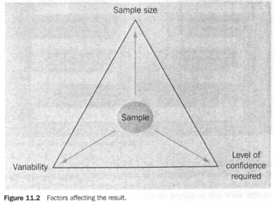
Statistical inference draws upon the probability results as developed in Part 3, especially from the Normal distribution. It can be shown that, given a few basic conditions, the statistics derived from a sample will follow a Normal distribution. To understand statistical inference it is necessary to recognize that three basic factors will affect our results; these are: the size of the sample the variability in the relevant population the level of confidence we wish to have in the results.

As illustrated in Figure 11.2, these three factors tend to pull in opposite directions and the final sample may well be a compromise between the factors. Increases in sample size will generally make the results more accurate (i.e. closer to the results which would be obtained from a census), but this is not a simple linear relationship so that doubling the sample size does not double the level of accuracy. Very small samples, for example under 30, tend to behave in a slightly different way from larger samples and we will look at this when we consider the use of the t-distribution. In practice, sample sizes can range from about 30 to 3000. Many national samples for market research or political opinion polling require a sample size of about 1000. Increasing sample size, also increases cost.

If there was no variation in the original population, then it would only be necessary to take a sample of one; for example, if everyone in the country had the same opinion about a certain government policy, then knowing the opinion of one individual would be enough. However, we do not live in such a homogeneous (boring) world, and there are likely to be a wide range of opinions on such issues as government policy. The design of the sample will need to ensure that the full range of opinions is represented. Even items which are supposed to be exactly alike turn out not to be so, for example, items coming off the end of a production line should be identical but there will be slight variations due to machine wear, temperature variation, quality of raw materials, skill of the operators, etc.

Since we cannot be 100% certain of our results, there will always be a risk that we will be wrong; we therefore need to specify how big this risk will be. Do you want to be 99% certain you have the right answer, or would 95% certain be sufficient? How about 90% certain? As we will see in this chapter, the higher the risk you are willing to accept of being wrong, the less exact the answer is going to be, and the lower the sample size needs to be.

11.2 Inference about a population
Calculations based on a sample are referred to as sample statistics. The mean and standard deviation, for example, calculated from sample information, will often be referred to as the sample mean and the sample standard deviation, but if not, should be understood from their context. The values calculated from population or census information are often referred to as population parameters. If all persons or items are included, there should be no doubt about these values (no sampling variation) and these values (population statistics) can be regarded as fixed within the particular problem context. (This may not mean that they are 'correct' since asking everyone is no guarantee that they will all tell the truth!)

If you have access to the web, try looking at the spreadsheet sampling.xls which takes a very small population (of size 10) and shows every possible sample of size 2, 3 or 4. The basic population data is as follows: A quick calculation would tell you that the population parameters are as follows: Mean = 13; Standard deviation =

By clicking on the Answer tab, you can find that, for a sample of 2, the overall mean is 13, with an overall standard deviation of You may wish to compare these answers with those shown, theoretically, later in the chapter.

The overall variation for samples of 2 is shown by a histogram in Figure 11.3.

Look through the spreadsheet for the other answers. Can you find a pattern in the results?

As we are now dealing with statistics from samples and making inferences to populations we need a notational system to distinguish between the two. Greek letters will be used to refer to population parameters, µ (mu) for the mean and σ (sigma) for the standard deviation, and N for the population size, while ordinary (roman) letters will be used for sample statistics, for the mean, s for the standard deviation, and n for the sample size. In the case of percentages, Π is used for the population and p for the sample.

11.3 Confidence interval for the population mean
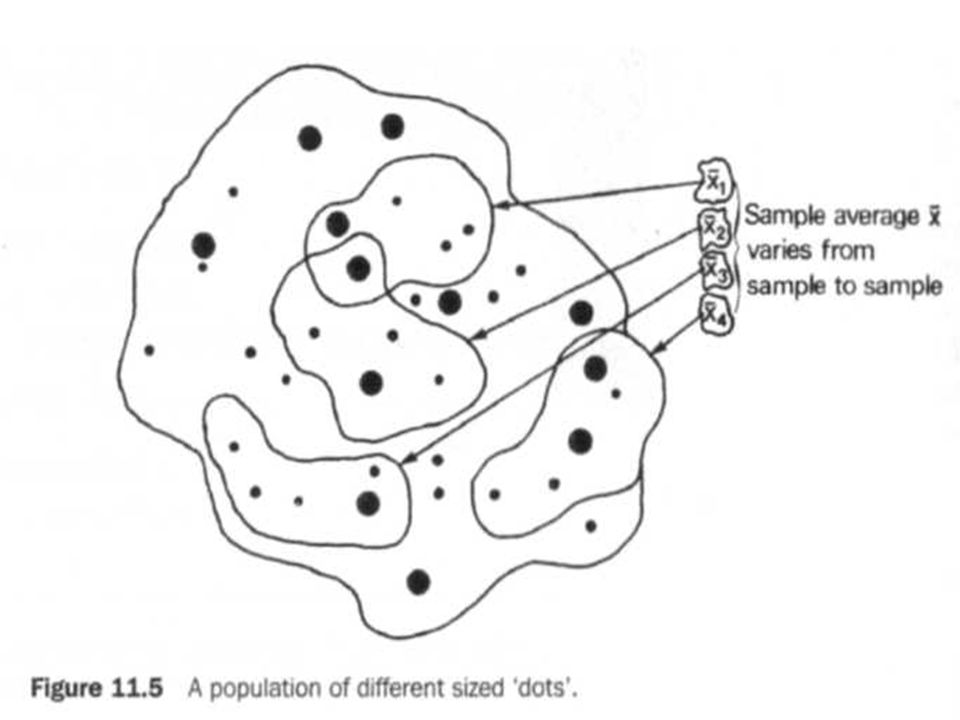
When a sample is selected from a population, the arithmetic mean may be calculated in the usual way, dividing the sum of the values by the size of the sample. If a second sample is selected, and the mean calculated, it is very likely that a different value for the sample mean will be obtained. Further samples will yield more (different) values for the sample mean. Note that the population mean is always the same throughout this process, it is only the different samples which give different answers. This is illustrated in Figure 11.5.

Since we are obtaining different answers from each of the samples, it would not be reasonable to just assume that the population mean was equal to any of the sample means. In fact each sample mean is said to provide a point estimate for the population mean, but it has virtually no probability of being exactly right; if it were, this would be purely by chance. We may estimate that the population mean lies within a small interval around the mean; this interval represents the sampling error.

Thus the population mean is estimated to lie in the region: ± sampling error Thus, we are attempting to create an interval estimate for the population mean.

You should recall from Chapter 10 that the area under a distribution curve can be used to represent the probability of a value being within an interval. We are therefore in a position to talk about the population mean being within the interval with a calculated probability. As we have seen in Section 10.4, the distribution of all sample means will follow a normal distribution, at least for large samples, with a mean equal to the population mean and a standard deviation equal to σ/√n.

The central limit theorem (for means) states that if a simple random sample of size n (n > 30) is taken from a population with mean µ and a standard deviation σ, the sampling distribution of the sample mean is approximately Normal with mean µ and standard deviation σ/√n. This standard deviation is usually referred to as the standard error when we are talking about the sampling distribution of the mean. This is a more general result than that shown in Chapter 10, since it does not assume anything about the shape of the population distribution; it could be any shape.

Compare this to the result of the sampling.xls spreadsheet. There and the standard deviation obtained from all samples was , but remember that here the sample size was only 2. The spreadsheet result is intended only to illustrate that the standard deviation for the distribution of sample means is lower than the population standard deviation.

From our knowledge of the Normal distribution (see Chapter 10 or Appendix C) we know that 95% of the distribution lies within 1.96 standard deviations of the mean. Thus, for the distribution of sample means, 95% of these will lie in the interval as shown in Figure 11.6.

This may also be written as a probability statement: This is a fairly obvious and uncontentious statement which follows directly from the central limit theorem. As you can see, a larger sample size would narrow the width of the interval (since we are dividing by root n). If we were to increase the percentage of the distribution included, by increasing the 0.95, we would need to increase the 1.96 values, and the interval would get wider.

By rearranging the probability statement we can produce a 95% confidence interval for the population mean: This is the form of the confidence interval which we will use, but it is worth stating what it says in words: the true population mean (which we do not know) will lie within 1.96 standard errors of the sample mean with a 95% level of confidence.

In practice you would only take a single sample, but this result utilizes the central limit theorem to allow you to make the statement about the population mean. There is also a 5% chance that the true population mean lies outside this confidence interval, for example, the data from sample 3 in Figure 11.7.

Case study 4 In the Arbour Housing Survey (see Case 4) 100 respondents had mortgages, paying on average £253 per month. If it can be assumed that the standard deviation for mortgages in the area of Tonnelle is £70, calculate a 95% confidence interval for the mean. The sample size is n = 100, the sample mean, = 253 and the population standard deviation, σ = 70.

Case study 4 By substituting into the formula given above, we have We are fairly sure (95% confident) that the average mortgage for the Tonnelle area is between £ and £ There is a 5% chance that the true population mean lies outside of this interval.

So far our calculations have attempted to estimate the unknown population mean from the known sample mean using a result found directly from the central limit theorem. However, looking again at our formula, we see that it uses the value of the population standard deviation, σ, and if the population mean is unknown it is highly unlikely that we would know this value. To overcome this problem we may substitute the sample estimate of the standard deviation, s, but unlike the examples in Chapter 5, here we need to divide by [n - 1) rather than n in the formula. This follows from a separate result of sampling theory which states that the sample standard deviation calculated in this way is a better estimator of the population standard deviation than that using a divisor of n. (Note that we do not intend to prove this result which is well documented in a number of mathematical statistics books.)

The structure of the confidence interval is still valid provided that the sample size is fairly large. Thus the 95% confidence interval which we shall use will be: For a 99% confidence interval, the formula would be:

As this last example illustrates, the more certain we are of the result (i.e. the higher the level of confidence), the wider the interval becomes. That is, the sampling error becomes larger. Sampling error depends on the probability excluded in the extreme tail areas of the Normal distribution, and so, as the confidence level increases, the amount excluded in the tail areas becomes smaller. This example also illustrates a further justification for sampling, since the measurement itself is destructive (length of life), and thus if all items were tested, there would be none left to sell.

11.3.1 Confidence intervals using survey data
It may well be the case that you need to produce a confidence interval on the basis of tabulated data. Case study The following example uses the table produced in the Arbour Housing Survey (and reproduced as Table 11.1) showing monthly rent.

Table Monthly rent Rent Frequency Under £50 7 £50 but under £100 12 £100 but under £150 15 £150 but under £200 30 £200 but under £250 53 £250 but under £300 38 £300 but under £400 20 £400 or more 5

We can calculate the mean and sample standard deviation using

The sample standard deviation, s, sometimes denoted by , is being used as an estimator of the population standard deviation σ. The sample standard deviation will vary from sample to sample in the same way that the sample mean, , varies from sample to sample. The sample mean will sometimes be too high or too low, but on average will equal the population mean µ You will notice that the distribution of sample means in Figure 11.6 is symmetrical about the population mean µ.

In contrast, if we use the divisor n, the sample standard deviation will on average be less than σ. To ensure that the sample standard deviation is large enough to estimate the population standard deviation σ reasonably, we use the divisor (n — 1). The calculations are shown in Tables 11.2 and 11.3. Confidence intervals are obtained by the substitution of sample statistics, from either Table 11.2 or 11.3 into the expression for the confidence interval.

Table 11.2 Rent Frequency x fx f (x - x)2 Under £50 7 25- 175
£50 but under £100 12 75 900 £100 but under £150 15 125 1875 £150 but under £200 30 L75 5250 £200 but under £250 53 225 11925 £250 but under £300 38 275 10 450 £300 but under £400 20 350 7 000 £400 or more 5 450* 2 250 180 39825

Table 11.3 Rent Frequency x fx fx2 Under £50 7 25- 175 4375
£50 but under £100 12 75 900 67 500 £100 but under £150 15 125 1875 234375 £150 but under £200 30 L75 5250 £200 but under £250 53 225 11925 £250 but under £300 38 275 10 450 £300 but under £400 20 350 7 000 £400 or more 5 450* 2 250 180 39825

The 95% confidence interval is:

Sample size for a mean As we have seen, the size of the sample selected has a significant bearing on the actual width of the confidence interval that we are able to calculate from the sample results. If this interval is too wide, it may be of little use, for example for a confectionery company to know that the weekly expenditure on a particular type of chocolate was between £0.60 and £3.20 would not help in planning. Users of sample statistics require a level of accuracy in their results.

Sample size for a mean From our calculations above, the confidence interval is given by: where z is the value from the Normal distribution tables (for a 95% interval this is 1.96). We could re-write this as: and now From this we can see that the error, e, is determined by the z value, the standard deviation and the sample size. As the sample size increases, so the error decreases, but to halve the error we would need to quadruple the sample size (since we are dividing by the square root of n).

11.3.2 Sample size for a mean Rearranging this formula gives:
and we thus have a method of determining the sample size needed for a specific error level, at a given level of confidence. Note that we would have to estimate the value of the sample standard deviation, either from a previous survey, or from a pilot study.

11.3.2 Sample size for a mean Example
What sample size would be required to estimate the population mean for a large set of company invoices to within £0.30 with 95% confidence, given that the estimated standard deviation of the value of the invoices is £5. To determine the sample size for a 95% confidence interval, let z = 1.96 and, in this case, e = £0.30 and s = £5. By substitution, we have: and we would need to select 1068 invoices to be checked, using a random sampling procedure.

11.4 Confidence interval for a population percentage
In the same way that we have used the sample mean to estimate a confidence interval for the population mean (µ) we can now use the percentage with a certain characteristic in a sample (p) to estimate the percentage with that characteristic in the whole population (Π). Sample percentages will vary from sample to sample from a given population (in the same way that sample means vary), and for large samples, this will again be in accordance with the central limit theorem.

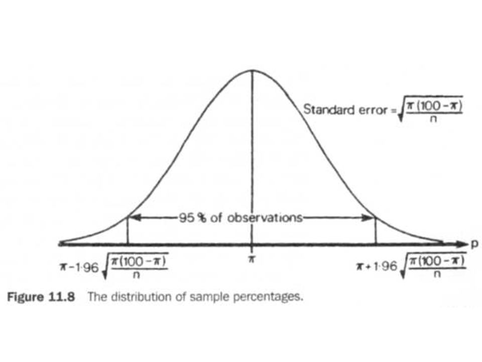
For percentages, this states that if a simple random sample of size n (n > 30) is taken from a population with a percentage Π having a particular characteristic, then the sampling distribution of the sample percentage, p, is approximated by a Normal distribution with a mean of Π and a standard error of

The 95% confidence interval for a percentage will be given by: as shown in Figure 11.8.

The probability statement would be: but a more usable format is:

Unfortunately, this contains the value of the population percentage, Π, on the right-hand side of the equation, and this is precisely what we are trying to estimate. Therefore we substitute the value of the sample percentage, p. Therefore the 95% confidence interval that we will use, will be given by:

A 99% confidence interval for a percentage would be given by: Interpretation of these confidence intervals is exactly the same as the interpretation of confidence intervals for the mean.

Example A random sample of 100 invoices has been selected from a large file of company records. If nine were found to contain errors, calculate a 95% confidence interval for the true percentage of invoices from this company containing errors. The sample percentage is p = 9%. This sample statistic is used to estimate the population percentage containing errors, Π.

By substituting into the formula for a 95% confidence interval, we have: we could write: or we could write: 3.391 < Π < As you can see, this is rather a wide interval.

11.4.1 Sample size for a percentage
As with the confidence interval for the mean, when we are considering percentages, we will often wish to specify the amount of acceptable error in the final result. If we look at the form of the error, we will be able to determine the appropriate sample size. The error is given by: and rearranging this gives: The value of p used will either be a reasonable approximation or a value from a previous survey or from a pilot study.

Example In a pilot survey, 100 invoices are selected randomly from a large file and nine were found to contain errors. What sample size would it be necessary to take if we wish to produce an estimate of the percentage of all invoices with errors to within plus or minus 3% with a 95% level of confidence? Here we may use the result of the pilot study, p = 9%. The value of z will be 1.96.

Substituting into the formula, we have: So, to achieve the required level of accuracy, we need a sample of 350 randomly selected invoices.

Where no information is available about the appropriate value of p to use in the calculations, we would use a value of 50%. Looking at the information given in Table 11.4, we can see that at a value of p = 50% we have the largest possible standard error, and thus the largest sample size requirement. This will be the safest approach where we have no prior knowledge.

Example What sample size would be required to produce an estimate for a population percentage to within plus or minus 3% if no prior information were available? In this case we would let p = 50% and assume the 'worst possible case'. By substituting into the formula, we have: So, to achieve the required accuracy, we would need a random sample of 1068.

Comparing the last two examples, we see that in both cases the level of confidence specified is 95%, and that the level of acceptable error to be allowed is plus or minus 3%. However, because of the different assumption that we were able to make about the value of p in the formula, we arrive at very different values for the required sample size. This shows the enormous value of having some prior information, since, for the cost of a small pilot survey we are able to reduce the main sample size to approximately 35% of the size it would have been without that information. In addition a pilot survey also allows us to test the questionnaire to be used (as discussed in Chapter 3).

An alternative to the usual procedure of a pilot survey followed by the main survey is to use a sequential sampling procedure. This involves a relatively small sample being taken first, and then further numbers are added as better and better estimates of the parameters become available. In practice, sequential sampling requires the continuation of interviews until results of sufficient accuracy have been obtained.

11.5 The difference between independent samples
We have so far considered only working with a single sample. In many cases of survey research we also wish to make comparisons between groups in the population, or between seemingly different populations. In other words, we want to make comparisons between two sets of sample results. This could, for example, be to test a new machining process in comparison to an existing one by taking a sample of output from each. Similarly we may want to compare consumers in the north with those in the south of a country or region.

In this section we will make these comparisons by calculating the difference between the sample statistics derived from each sample. We will also assume that the two samples are independent and that we are dealing with large samples. (For information on dealing with small samples see Section 11.7.) Although we will not derive the statistical theory behind the results we use, it is important to note that the theory relies on the samples being independent and that the results do not hold if this is not the case.

For example, if you took a single sample of people and asked them a series of questions, and then two weeks later asked the same people another series of questions, the samples would not be independent and we could not use the confidence intervals shown in this section. (You may recall from Chapter 3 that this methodology is called a panel survey.) One result from statistical sampling theory states that although we are taking the difference between the two sample parameters (the means or percentages), we add the variances. This is because the two parameters are themselves variable and thus the measure of variability needs to take into account the variability of both samples.

11.5.1 Confidence interval for the difference of means
The format of a confidence interval remains the same as before: population parameter = sample statistic ± sampling error but now the population parameter is the difference between the population means (µ1-µ2), the sample statistic is the difference between the sample means and the sampling error consists of the z-value from the Normal distribution tables multiplied by the root of the sum of the sample variances divided by their respective sample sizes. This sounds like quite a mouthful (!) but is fairly straightforward to use with a little practice.

The 95% confidence interval for the difference of means is given by the following formula: where the subscripts denote sample 1 and sample 2. (Note the relatively obvious point that we must keep a close check on which sample we are dealing with at any particular time.)

Case study It has been decided to compare some of the results from the Arbour Housing Survey with those from the Pelouse Housing Survey. Of particular interest was the level of monthly rent, a summary of which is given below:

As this range includes zero, we cannot be 95% confident that there is a difference in rent between the two areas, even though the average rent on the basis of sample information is higher in Tonnelle (the area covered by the Arbour Housing Survey). The observed difference could be explained by inherent variation in sample results.

11.5.2 Confidence interval for the difference of percentages
In this case we only need to know the two sample sizes and the two sample percentages to be able to estimate the difference in the population percentages. The formula for this confidence interval takes the following form: where the subscripts denote sample 1 and sample 2.

Case study In the Arbour Housing Survey, 234 respondents out of the 300 reported that they had exclusive use of a flush toilet inside the house. In the Pelouse Housing Survey, 135 out of 150 also reported that they had exclusive use of a flush toilet inside the house. Construct a 95% confidence interval for the percentage difference in this housing quality characteristic. The summary statistics are as follows: The Arbour Housing Survey The Pelouse Housing Survey (Survey 1) (Survey 2) n1 = n2 = 150 p1 = 234/300 x 100 = 78% p2 = 135/150 x 100 = 90%

By substitution, the 95% confidence interval is: This range does not include any positive value or zero, suggesting that the percentage from the Arbour Housing Survey is less than that from the Pelouse Housing Survey. In the next chapter we will consider how to test the 'idea' that a real difference exists. For now, we can accept that the sample evidence does suggest such a difference.

The significance of the results will reflect the sample design. The width of the confidence interval (and the chance of including a zero difference) will decrease as: the size of sample or samples is increased the variation is less (a smaller standard deviation) in the case of percentages, the difference from 50% increases (see Table 11.4); and the sample design is improved (e.g. the use of stratification). The level of confidence still needs to be chosen by the user - 95% being most typical. However, it is not uncommon to see the use of 90%, 99% and 99.9% confidence intervals.

11.6 The finite population correction factor
In all the previous sections of this chapter we have assumed that we are dealing with samples that are large enough to meet the conditions of the central limit theorem (n > 30), but are small relative to the defined population. We have seen (Section ), for example (making these assumptions), that a sample of just over 1000 is needed to produce a confidence interval with a sampling error of ±3%. However, suppose the population were only a 1000, or 1500 or 2000? Some populations by their nature are small, e.g. specialist retail outlets in a particular region. In some cases we may decide to conduct a census and exclude sampling error. In other cases we may see advantages in sampling.

As the proportion of the population included in the sample increases, the sampling error will decrease. Once we include all the population in the sample - take a census - there will be no error due to sampling (although errors may still arise due to bias, lying, mistakes, etc.). To take this into account in our calculations we need to correct the estimate of the standard error by multiplying it by the finite population correction factor.

This is given by the following formula: where n is the sample size, and N is the population size. As you can see, as the value of n approaches the value of N, the value of the bracket gets closer and closer to zero, thus making the size of the standard error smaller and smaller. As the value of n becomes smaller and smaller in relation to N, the value of the bracket gets nearer and nearer to one, and the standard error gets closer and closer to the value we used previously.

Where the finite population correction factor is used, the formula for a 95% confidence interval becomes:

Example Suppose a random sample of 30 wholesalers used by a toy producer order, on average cartons of crackers each year. The sample showed a standard deviation of 1500 cartons. In total, the manufacturer uses 40 wholesalers. Find a 95% confidence interval for the average size of annual order to this manufacturer.

Here, n = 30, N = 40, x = and s = 1500. Substituting these values into the formula, we have: which we could write as: If no allowance had been made for the high proportion of the population selected as the sample, the 95% confidence interval would have been: <M< which is considerably wider and would make planning more difficult.

As a 'rule of thumb', we only consider using the finite correction factor if the sample size is 10% or more of the population size. Typically, we don't need to consider the use of this correction factor, because we work with relatively large populations. However, it is worth knowing that 'correction factors' do exist and are seen as a way of reducing sampling error.

11.7 The t-distribution We have been assuming that either the population standard deviation (σ) was known (an unlikely event), or that the sample size was sufficiently large so that the sample standard deviation, s, provided a good estimate of the population value (see Section ). Where these criteria are not met, we are not able to assume that the sampling distribution is a Normal distribution, and thus the formulae developed so far will not apply. As we have seen in Section , we are able to calculate the standard deviation from sample data, but where we have a small sample, the amount of variability will be higher, and as a result, the confidence interval will need to be wider.

11.7 The t-distribution If you consider the case where there is a given amount of variability in any population, when a large sample is taken, it is likely to pick up examples of both high and low values, and thus the variability of the sample will reflect the variability of the population. When a small sample is taken from the same population, the fewer values available make it less likely that all of the variation is reflected in the sample. Thus a given standard deviation in the small sample would imply more variability in the population than the same standard deviation in a large sample.

11.7 The t-distribution Even with a small sample, if the population standard deviation is known, then the confidence intervals can be constructed using the Normal distribution as: where z is the critical value taken from the Normal distribution tables.

11.7 The t-distribution Where the value of the population standard deviation is not known we will use the t-distribution to calculate a confidence interval: where t is a critical value from the t-distribution. (The derivation of why the t -distribution applies to small samples is beyond the scope of this book, and of most first-year courses, but the shape of this distribution as described below gives an intuitive clue as to its applicability.)

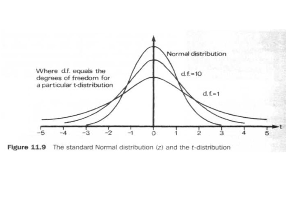
11.7 The t-distribution The shape of the t-distribution is shown in Figure 11.9. You can see that it is still a symmetrical distribution about a mean (like the Normal distribution), but that it is wider. In fact it is a misnomer to talk about the t-distribution, since the width and height of a particular t -distribution varies with the number of degrees of freedom. This new term is related to the size of the sample, being represented by the letter v (pronounced new), and is equal to n - 1 (where n is the sample size). As you can see from the diagram, with a small number of degrees of freedom, the t-distribution is wide and flat; but as the number of degrees of freedom increases, the t-distribution becomes taller and narrower.

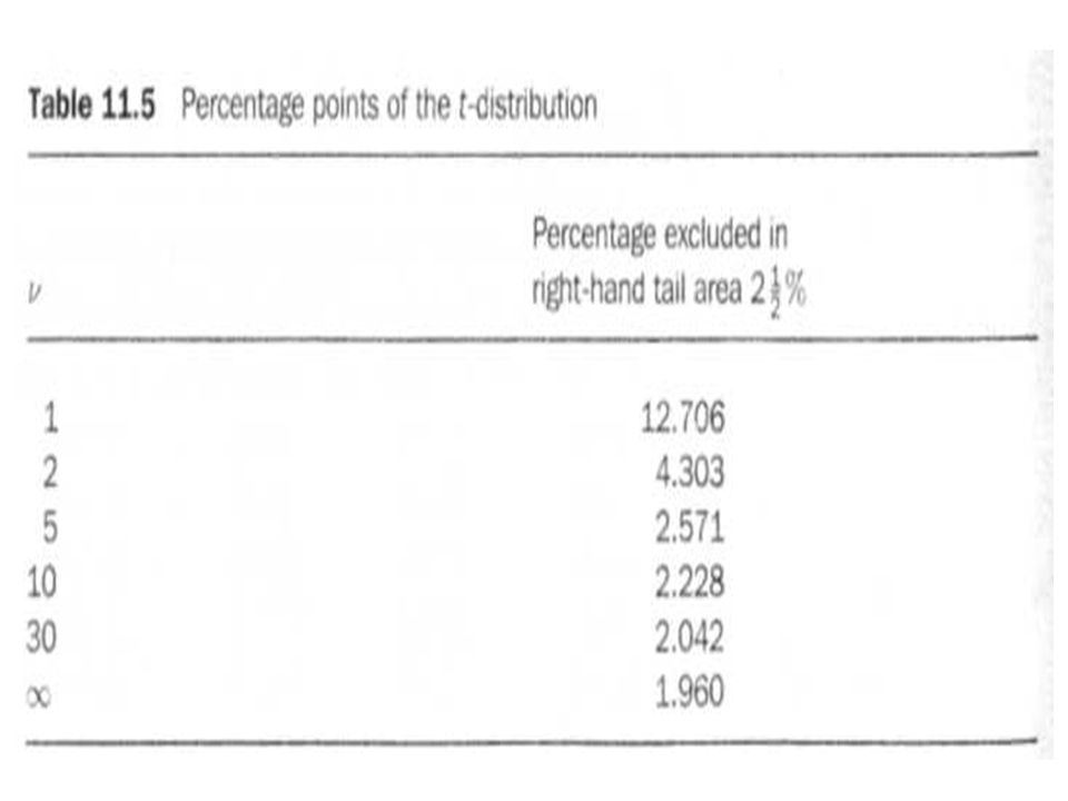
11.7 The t-distribution As the number of degrees of freedom increases, the t-distribution tends to the Normal distribution. Values of the t-distribution are tabulated by degrees of freedom and are shown in Appendix D but, to illustrate the point about the relationship to the Normal distribution, consider Table 11.5. We know that to exclude 2.5% of the area of a Normal distribution in the right-hand tail we would use a z-value of 1.96. Table 11.5 shows the comparative values of t for various degrees of freedom.

11.7 The t-distribution Before using the t-distribution, let us consider an intuitive explanation of degrees of freedom. If a sample were to consist of one observation we could estimate the mean (take the average to be that value), but could make no estimate of the variation. If the sample were to consist of two observations, we would have only one measure of difference or one degree of freedom. If the sample consisted of three values, then we would have two estimates of difference, or two degrees of freedom.

11.7 The t-distribution Degrees of freedom can be described as the number of independent pieces of information. In estimating variation around a single mean the degrees of freedom will be n - 1. If we were estimating the variation around a line on a graph (see Section 15.5) the degrees of freedom would be n - 2 since two parameters have been estimated to position the line.

11.7 The t-distribution The 95% confidence interval for the mean from sample data when σ is unknown takes the form: where t0.025 excludes 2.5% of observations in the extreme right-hand tail area.

11.7 The t-distribution Example
A sample of six representatives were selected from a large group to estimate their average daily mileage. The sample mean was 340 miles and the standard deviation 60 miles. Calculate the 95% confidence interval for the population mean. The summary statistics are: n = 6, = 340, and s = 60. In this case, the degrees of freedom are v - n - 1 = 5, and the critical value from the t-distribution is (see Appendix D).

11.7 The t-distribution By substitution, the 95% confidence interval is: If the sampling error is unacceptably large we would need to increase the size of the sample.

11.7 The t-distribution We have illustrated the use of the t-distribution for estimating the 95% confidence interval for a population mean from a small sample. Similar reasoning will allow calculation of a 95% confidence interval for a population percentage from a single sample, or variation of the level of confidence by changing the value of t used in the calculation. Where two small independent samples are involved, and we wish to estimate the difference in either the means or the percentages, we can still use the t-distribution, but now the number of degrees of freedom will be related to both sample sizes:

11.7 The t-distribution and it will also be necessary to allow for the sample sizes in calculating a pooled standard error for the two samples. In the case of estimating a confidence interval for the difference between two means the pooled standard error is given by:

11.7 The t-distribution and the confidence interval is:
the t value being found from the tables, having degrees of freedom. A theoretical requirement of this approach is that both samples have variability of the same order of magnitude.

11.7 The t-distribution Example
Two processes are being considered by a manufacturer who has been able to obtain the following figures relating to production per hour. Process A produced units per hour as the average from a sample of 10 hourly runs. The standard deviation was 4. Process B had 15 hourly runs and gave an average of units per hour, with a standard deviation of 3.

11.7 The t-distribution The summary statistics are as follows:
Thus the pooled standard error for the two samples is given by

11.7 The t-distribution There are v = = 23 degrees of freedom, and for a 95% confidence interval, this gives a t-value of (see Appendix D). Thus the 95% confidence interval for the difference between the means of the two processes is

11.8 Confidence interval for the median – large sample approximation
As we have seen in Chapter 5, the arithmetic mean is not always an appropriate measure of average. Where this is the case, we will often want to use the median. (To remind you, the median is the value of the middle item of a group, when the items are arranged in either ascending or descending order.) Reasons for using a median may be that the data is particularly skewed, for example income or wealth data, or it may lack calibration, for example the ranking of consumer preferences. Having taken a sample, we still need to estimate the errors or variation due to sampling and to express this in terms of a confidence interval, as we did with the arithmetic mean.

Since the median is determined by ranking all of the observations and then counting to locate the middle item, the probability distribution is discrete (the confidence interval for a median can thus be determined directly using the binomial distribution). If the sample is reasonably large (n > 30), however, a large sample approximation will give adequate results (see Chapter 10 for the Normal approximation to the binomial distribution).

Consider the ordering of observations by value, as shown below: X1 ,X2 , X3 ,…. , Xn where Xi ≤ Xi+1 . The median is the middle value of this ordered list, corresponding to the (n + 1)/2 observation. The confidence interval is defined by an upper ordered value (u) and a lower ordered value (l).

For a 95% confidence interval, these values are located using: where n is the sample size.

Example Suppose a random sample of 30 people has been selected to determine the median amount spent on groceries in the last seven days. Results are listed in the table below: 2.5 2.7 3.45 5.72 6.1 6.18 7.58 8.42 8.9 9.14 9.4 10.31 11.4 11.55 11.9 12.14 12.3 12.6 14.37 15.42 17.51 19.2 22.3 30.41 31.43 42.44 54.2 59.37 60.21 65.27

The median will now correspond to the (30 + l)/2 = 15.5th observation. Its value is found by averaging the 15th and 16th observations: median= The sample median is a point estimate of the population median. A 95% confidence interval is determined by locating the upper and lower boundaries.

thus the upper bound is defined by the 21st value (rounding up) and the lower bound by the 10th value (rounding down).

By counting through the set of sample results we can find the 95% confidence interval for the median to be: 9.14 < median < 17.51 This is now an interval estimate for the median.

Applied Quantitative Methods MBA course Montenegro

Similar presentations

Presentation on theme: "Applied Quantitative Methods MBA course Montenegro"— Presentation transcript:

Similar presentations

About project

Feedback

Log in

Auth with social network:

Applied Quantitative Methods MBA course Montenegro

Similar presentations

Presentation on theme: "Applied Quantitative Methods MBA course Montenegro"— Presentation transcript:

Similar presentations

About project

Feedback