1. Theory of wind-driven sea by V.E. Zakharov S. Badulin A.Dyachenko V.Geogdjaev N.Ivenskykh A.Korotkevich A.Pushkarev In collaboration with:

2. Plan of the lecture: 1.Weak-turbulent theory 2.Kolmogorov-type spectra 3.Self-similar solutions 4.Experimental verification of weak-turbulent theory 5.Numerical verification of weak-turbulent theory 6.Freak-waves solitons and modulational instability

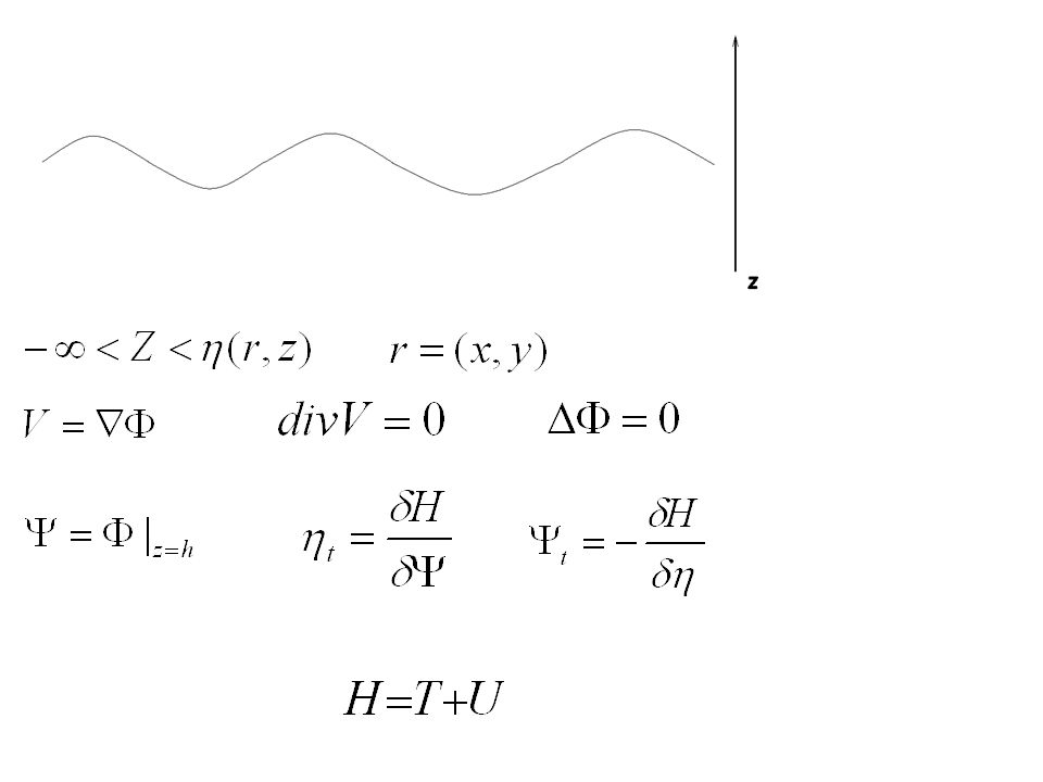
4. - Green function of the Dirichlet-Neuman problem -- average steepness

5. Normal variables: Truncated equations:

6. Canonical transformation - eliminating three-wave interactions:

7. where

8. Statistical description: Hasselmann equation:

9. Kinetic equation for deep water waves (the Hasselmann equation, 1962) - empirical dependences

10. Conservative KE has formal constants of motion wave action energy momentum Q – flux of action P – flux of energy For isotropic spectra n=n(|k|) Q and P are scalars let n ~ k -x, then S nl ~ k 19/2-3x F(x), 3 < x < 9/2

11. Energy spectrum

12. F(x)=0, when x=23/6, x=4 – Kolmogorov-Zakharov solutions Kolmogorov’s constants are expressed in terms of F(y), where exponent for y F(y)

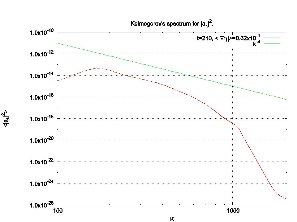
13. Kolmogorov’s cascades S nl =0 (Zakharov, PhD thesis 1966) Direct cascade (Zakharov PhD thesis,1966; Zakharov & Filonenko 1966) Inverse cascade (Zakharov PhD thesis,1966 ) Numerical experiment with “artificial” pumping (grey). Solution is close to Kolmogorov-Zakharov solutions in the corresponding “inertial” intervals

14. Phillips, O.M., JFM. V.156,505-531, 1985.

15. S nl >> S input, S diss Nonlinear transfer dominates! Just a hypothesis to check

16. Existence of inertial intervals for wind-driven waves is a key point of critics of the weak turbulence approach for water waves Wave input term S in for U 10  p /g=1 Non-dimensional wave input rates Dispersion of different estimates of wave input S in and dissipation S diss is of the same magnitude as the terms themselves !!!

17. Term-to-term comparison of S nl and S in. Algorithm by N. Ivenskikh (modified Webb-Resio-Tracy). Young waves, standard JONSWAP spectrum Mean-over-angle Down-wind

18. The approximation procedure splits wave balance into two parts when S nl dominates We do not ignore input and dissipation, we put them into appropriate place ! Self-similar solutions (duration-limited) can be found for (*) for power-law dependence of net wave input on time

19. We have two-parametric family of self-similar solutions where relationships between parameters are determined by property of homogeneity of collision integral S nl and function of self-similar variable U   obeys integro-differential equation Stationary Kolmogorov-Zakharov solutions appear to be particular cases of the family of non-stationary (or spatially non-homogeneous) self-similar solutions when left-hand and right-hand sides of (**) vanish simultaneously !!!

20. Self-similar solutions for wave swell (no input and dissipation)

21. Quasi-universality of wind-wave spectra Spatial down-wind spectra  spectra Dependence of spectral shapes on indexes of self-similarity is weak

22. Numerical solutions for duration-limited case vs non-dimensional frequency    U/g *

23. 1. Duration-limited growth 2. Fetch-limited growth Time-(fetch-) independent spectra grow as power-law functions of time (fetch) but experimental wind speed scaling is not consistent with our “spectral flux approach” Experimental dependencies use 4 parameters. Our two-parameteric self- similar solutions dictate two relationships between these 4 parameters For case 2  ss – self-similarity parameter

24. Thanks to Paul Hwang Experimental power-law fits of wind-wave growth. Something more than an idealization?

25. Exponents are not arbitrary, not “universal”, they are linked to each other. Numerical results (blue – “realistic” wave inputs) Total energy and total frequency Energy and frequency of spectral “core”

26. Exponents p  (energy growth) vs q  (frequency downshift) for 24 fetch- limited experimental dependencies. Hard line – theoretical dependence p  =(10q  -1)/2 1.“Cleanest” fetch- limited 2.Fetch-limited composite data sets 3.One-point measurements converted to fetch- limited one 4.Laboratory data included

27. Self-similarity parameter  ss vs exponent p  for 24 experimental fetc-limited dependencies 1.“Cleanest” fetch- limited 2.Fetch-limited composite data sets 3.One-point measurements converted to fetch- limited one 4.Laboratory data included

28. Numerical verification of the Hasselmann equation

29. Dynamical equations : Hasselmann (kinetic) equation :

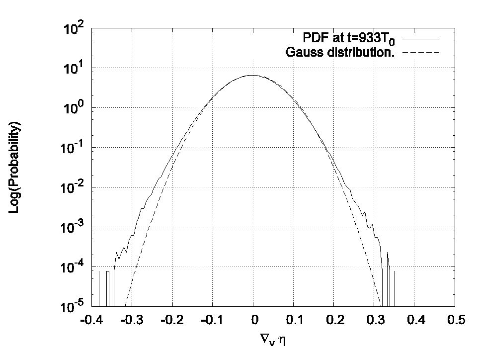
30. Two reasons why the weak turbulent theory could fail: 1.Presence of the coherent events -- solitons, quasi - solitons, wave collapses or wave- breakings 2.Finite size of the system – discrete Fourier space: Quazi-resonances

31. Dynamic equations: domain of 4096x512 point in real space Hasselmann equation: domain of 71x36 points in frequency-angle space

32. Four damping terms: 1. Hyper-viscous damping 2. WAM cycle 3 white-capping damping 3. WAM cycle 4 white-capping damping 4. New damping term

33. WAM Dissipation Function: WAM cycle 3: WAM cycle 4: Komen 1984 Janssen 1992 Gunter 1992 Komen 1994

48. New Dissipation Function:

50. Freak-waves solitons and modulational instability