1. Matlab exercise 101071041 計財 16 陳怡鳳

2. Plot BLS_P % PlotBLS.m S0 = 20:1:70; X = 50; r = 0.04; sigma = 0.4; for T=2:-0.25:0 [c,p]=blsprice(S0,X,r,T,sigma); plot(S0,p); hold on; end axis([20 70 -5 35]); grid on Question : 自己寫的 b-s model 即使用兩個迴圈還是無法跑 (?

3. Output 價外 s>50 價內 s<50 價平 =s50 ？

4. Option price= intrinsic value + time value Intrinsic value(for put) = Max(0,X-S) Time value = The value for waiting Time value may be negative For deep in the money only. More possible for put than call.

5. Plot the variation of theta with stock price for a call x=50; r=0.05; t=0.5; sig=0.2; div=0; s=30:120; [call_theta,put_theta]=blstheta(s,x,r,t,sig,div); figure plot(s,call_theta,'-') title('theta vs. s') xlabel('s') ylabel('theta') legend('theta of call')

7. Plot the variation of gamma with stock price for a call x=50; r=0.05; t=0.5; sig=0.2; div=0; s=30:120; gamma=blsgamma(s,x,r,t,sig,div); figure plot(s,gamma,'-') title('gamma vs. s') xlabel('s') ylabel('gamma') legend('gamma')

9. Plot the variation of vega with stock price for a call x=50; r=0.05; t=0.5; sig=0.2; div=0; s=30:120; vega=blsvega(s,x,r,t,sig,div); figure plot(s,vega,'-') title('vega vs. s') xlabel('s') ylabel('vega') legend('vega')

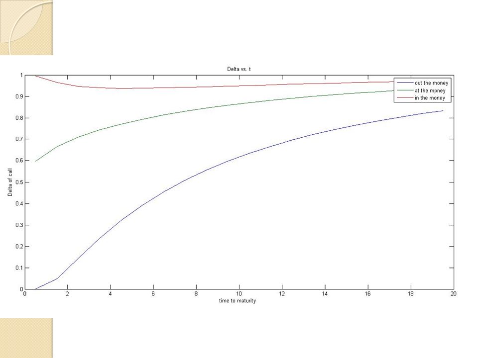
11. Plot the patterns for variation of delta with time to maturity for a call option x=50; r=0.05; t=0.5:20; sig=0.2; div=0; s1=30; [call_delta1,put_delta]=blsdelta(s1,x,r,t,sig,div); s2=50; [call_delta2,put_delta]=blsdelta(s2,x,r,t,sig,div); s3=70; [call_delta3,put_delta]=blsdelta(s3,x,r,t,sig,div); plot(t,call_delta1,'-',t,call_delta2,'-',t,call_delta3,'-') title('Delta vs. t') xlabel('time to maturity ') ylabel('Delta of call') legend('out the money','at the mpney','in the money')

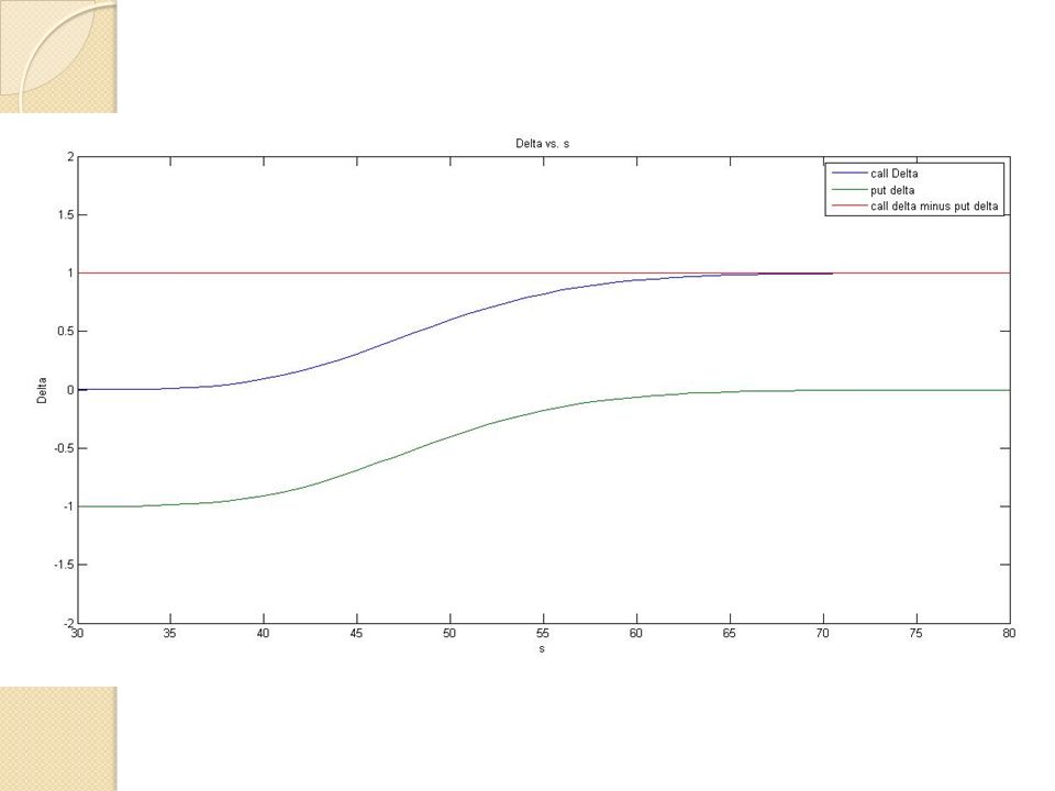
13. For interest _ call and put delta comparison x=50; r=0.05; t=0.5; sig=0.2; div=0; s=30:80; [call_delta,put_delta]=blsdelta(s,x,r,t,sig,div); change=call_delta-put_delta; figure plot(s,call_delta,'-',s,put_delta,'-',s,change,'-') title('Delta vs. s') xlabel('s') ylabel('Delta') legend('call Delta','put delta','call delta minus put delta') axis([30 80 -2 2]);