1. On the Heterogeneity, Stability and Validity of Risk Preference Measures Chetan Dave Catherine Eckel Cathleen Johnson Christian Rojas University of Texas at Dallas University of Arizona University of Massachusetts (Amherst) ESA, July, 2007

2. Measuring Preferences: Key Questions Are risk preferences stable across elicitation measures?  Since Slovic (1964), considerable evidence they are not Do risk preferences vary systematically by subject characteristics in the same way across measures?  (Gender, age, income) Does math ability affect elicited preferences?  Ability: Low/Medium/High Math Literacy Are risk preferences stable across time?  Two Datasets: Test Data vs. Re-Test Data

3. Motivation Lots of folks are working on heterogeneity in risk preferences  (many of them are here) There are lots of elicitation tasks, depending on the purpose of the study Our purpose: to develop a simple, easy to administer measure of individual risk preferences that can be used to “predict” or better understand individual choices.  Household decisions, human capital choices, technology adoption

4. Motivation, cont’d We compare two lottery choice methods (more on these soon) Non-student data set (collected for another purpose) Subjects complete both risk elicitation measures Survey, math literacy measure Subset of pre-selected subjects participated in a retest

5. The CSL Study Purpose: study barriers to post-secondary acquisition of human capital Data: lab experiments with non-traditional subject pool  ~900 adult participants in Canada (recruited, volunteers)  102 sessions  Ages 18-54 years  Urban and Non-Urban samples  156 participate in retest 6 months later Average earnings: CAD$165  Subjects paid for one decision chosen at random  100 decisions: 40 time pref; 32 risk and ambiguity; 28 financing for post-secondary education, max = $1000 grant, $5000 guaranteed loan

6. The CLS Study (cont’d.) Two experiments to elicit risk preferences:  Holt-Laury (2002) 10 binary choices between more and less risky gambles  Eckel-Grossman (2002) Choice of 1 from set of 6 50/50 gambles Discrete binary response data  0 = less risky choice  1 = more risky choice

7. Holt-Laury Task

8. Holt-Laury Summary Data Given a CRRA utility function for money (M) r U(M|r) = M1-r/(1-r)

9. Eckel-Grossman Task x

10. Eckel-Grossman Summary Data

11. Short Detour FAQ: How do you code Eckel-Grossman as a set of binary choices? Notice the gambles are ordered Increase linearly in risk and return as you go down the table One choice implies binary ordering

12. This person chooses Gamble 3 This implies 5 binary choices: 2 is preferred to 1 3 is preferred to 2 3 is preferred to 4 4 is preferred to 5 5 is preferred to 6

13. Comparison of Eckel-Grossman and Holt-Laury H-L: varying probabilities, constant payoffs E-G: constant probability, varying payoffs, all 50-50 gambles

15. The Numeracy Measure Subcomponent of the Educational Testing Service’s Adult Literacy and Lifeskills Survey (ALLS) 31 problems involving the use of mathematics in real-life situations. Low numeracy ≤ 1 standard dev. below average High numeracy ≥ 1 standard dev. above average

16. Model and Estimation Given a CRRA utility function for money (M) parameterized by  r U(M|r) = M 1-r /(1-r) Can construct a likelihood function L(r, ,|Y) where  measures ‘noise’ in binary risk choices (Y) r and  can also be made a function of observed characteristics of subjects

17. Results 1: Does the Elicitation Instrument Affect Estimates?

18. Estimates of CRRA Utility Function r = Coefficient of relative risk aversion  = Logit error parameter Differences significant at p = 0.000,  2 (1) = 52.62

19. Estimates of CRRA Utility (cont’d.) Eckel-Grossman and Holt-Laury give significantly different estimates of r “Ruler” affects measure! H-L has higher error parameter than E-G Why?

20. Results II: How do demographics and ability affect estimates ? IIA: Effect on preference parameters IIB: Effect on parameters and errors IIC: Are parameters stable across instruments?

21. Effect on preference parameters

22. Effect on Preference Parameters (cont’d.) Income, Age and Math Literacy are significant determinants (correlates) of preferences Low Income: more risk averse Young: less risk averse Low math score: appear more risk averse  Could this be due to greater errors?

23. Effect on Parameters and Errors

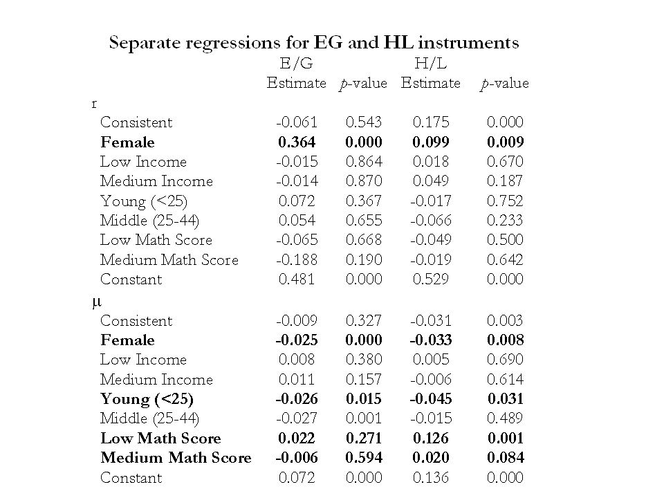
24. Effect on Parameters and Errors (cont’d)

25. IIB. Parameters and Errors (cont’d.) People who are consistent are more risk averse and have less noise (randomness) Young have less noise Lower numerical literacy increases randomness in risk parameters; appear more risk averse Females are more risk averse and have lower noise

26. IIIC: Parameter stability across measures Is the impact of gender, age, income similar across measures? Is the impact of math literacy similar across measures?

28. Distribution of noise parameter

29. How good are predictions? Calculate index: n is the number of decisions for the task (5 for Eckel-Grossman and 10 for Holt-Laury) ‘fraction’ variables represent the true and the predicted fraction of safe choices for decision i across all individuals. Holt-Laury task has indices of 0.79, 0.88 and 0.92 for low, medium and high math literacy subjects Eckel-Grossman instrument has a precision index of 0.81.

30. IIC: Comparison Women are substantially more risk averse in E/G; lower noise in both Young have lower noise in both Low math literacy affects noise in H/L only Noise parameter is similar to E/G for H/L high literacy, but higher for med and especially low literacy “Precision” is equivalent for high literacy, not for Medium or Low.

31. Results III: Are Preferences Stable Across Time? IIIA. Eckel-Grossman IIIB. Holt-Laury

32. IIIA. Stability of Eckel-Grossman EG Instrument EstimateStd. Err.p-value r  Re-test 0.0800.0900.377  Constant 0.4320.0610.000   Re-test -0.0320.0080.687  Constant 0.0520.0050.000 LogL:920.631 # obs1560

33. IIIB. Stability of Holt-Laury HL Instrument EstimateStd. Err.p-value r  Re-test 0.1180.0800.141  Constant 0.7070.0550.000   Re-test -0.0440.0280.122  Constant 0.1120.0200.000 LogL:1182.848 # obs3,120

34. Concluding Remarks Question # 1: Are preferences stable across measures used to elicit them?  Answer: A qualified No. Elicitation instruments do matter to an extent Question # 2: Do preference estimates by subject characteristics vary across measures?  Answer for Demographics: Yes

35. Concluding Remarks (cont’d.) Question #3: Are preference measures sensitive to math literacy:  Answer: Yes, H/L only Question # 4: Are preference measures stable across time?  Answer: Yes. But E-G does “better” than H-L Question #A1: Internal v. external validity?

36. Validity: Correlations of risk measures with “real” decisions.

37. Measuring preferences Need to develop instruments that are appropriate for population, purpose Finer screen v. accessibility tradeoff For literate population, no tradeoff For medium and low literate population, there may be a serious tradeoff! Considerable precision is lost with more complex instrument Important to take care with design for low- literacy populations

38. Ex: Next gen of instruments (risk)