Download presentation
Presentation is loading. Please wait.

1
Chapter 14 Simple Regression
Statistics for Business and Economics 6th Edition Chapter 14 Simple Regression

2
Chapter Goals After completing this chapter, you should be able to:
Explain the correlation coefficient and perform a hypothesis test for zero population correlation Explain the simple linear regression model Obtain and interpret the simple linear regression equation for a set of data Describe R2 as a measure of explanatory power of the regression model Understand the assumptions behind regression analysis

3
Correlation Analysis The population correlation coefficient is denoted ρ (the Greek letter rho) The sample correlation coefficient is where

4
Introduction to Regression Analysis
Regression analysis is used to: Predict the value of a dependent variable based on the value of at least one independent variable Explain the impact of changes in an independent variable on the dependent variable Dependent variable: the variable we wish to explain (因变量) (also called the endogenous variable) Independent variable: the variable used to explain (自变量) the dependent variable (also called the exogenous variable) 被预测变量称之为因变量,进行预测的变量为自变量。 在样本中我们只考虑两者的关系可以用一条直线近似表示出简单类型的回归分析,这种回归分析称之为简单线性回归,涉及两个或两个以上自变量的回归分析为多元回归分析。 简单线性回归方程描述了y的平均值或期望值是如何依赖x的。我们利用样本数据和最小二乘法求出估计回归方程,实际上bo和b1是用来估计模型中未知参数beita0和beita1的样本统计量。 为了估计回归方程拟合度,我们引入确定系数的概念。确定系数是因变量y中的变异能被估计回归方程所解释的部分所占的比例。
 (also called the endogenous variable) Independent variable: the variable used to explain (自变量) the dependent variable. (also called the exogenous variable) 被预测变量称之为因变量,进行预测的变量为自变量。 在样本中我们只考虑两者的关系可以用一条直线近似表示出简单类型的回归分析,这种回归分析称之为简单线性回归,涉及两个或两个以上自变量的回归分析为多元回归分析。 简单线性回归方程描述了y的平均值或期望值是如何依赖x的。我们利用样本数据和最小二乘法求出估计回归方程,实际上bo和b1是用来估计模型中未知参数beita0和beita1的样本统计量。 为了估计回归方程拟合度,我们引入确定系数的概念。确定系数是因变量y中的变异能被估计回归方程所解释的部分所占的比例。")
5
Linear Regression Model
The relationship between X and Y is described by a linear function Changes in Y are assumed to be caused by changes in X Linear regression population equation model Where 0 and 1 are the population model coefficients and is a random error term. 线性回归模型 is a random error term 为随机误差项的随机变量

6
Simple Linear Regression Model简单线性回归模型
The population regression model: Random Error term Population Slope Coefficient Population Y intercept Independent Variable Dependent Variable Linear component Random Error component

7
Simple Linear Regression Model
(continued) Y Observed Value of Y for Xi εi Slope = β1 Predicted Value of Y for Xi Random Error for this Xi value Intercept = β0 Xi X
 Y. Observed Value of Y for Xi. εi. Slope = β1. Predicted Value of Y for Xi. Random Error for this Xi value. Intercept = β0. Xi. X.")
8
Simple Linear Regression Equation简单线性回归方程
The simple linear regression equation provides an estimate of the population regression line Estimated (or predicted) y value for observation i Estimate of the regression intercept Estimate of the regression slope 简单线性回归方程 Yjian是y的估计值 观察值与估计值 Value of x for observation i The individual random error terms ei have a mean of zero
 y value for observation i. Estimate of the regression intercept. Estimate of the regression slope. 简单线性回归方程. Yjian是y的估计值. 观察值与估计值. Value of x for observation i. The individual random error terms ei have a mean of zero.")
9
回归分析不能看做是在变量间建立一个因果关系的过程,回归分析只能表明变量是如何或者以怎样的程度彼此联系在一起的。任何关于因果的结论必须建立在对个体或多个个体的有关应用的大量信息判断基础上的。

10
Least Squares Estimators 最小二乘法估计
b0 and b1 are obtained by finding the values of b0 and b1 that minimize the sum of the squared differences between y and : 最小二乘法是利用样本进行回归方程估计的一种方法,是通过使自变量y的观察值和估计值之间的离差平方和达到最小的方法,得到一个回归方程的估计。是选择能与样本数据有最好拟合的方程,是应用最广泛的方法。 Differential calculus is used to obtain the coefficient estimators b0 and b1 that minimize SSE

11
Least Squares Estimators
(continued) The slope coefficient estimator is And the constant or y-intercept is The regression line always goes through the mean x, y
 The slope coefficient estimator is. And the constant or y-intercept is. The regression line always goes through the mean x, y.")
12
Linear Regression Model Assumptions
The true relationship form is linear (Y is a linear function of X, plus random error) The error terms, εi are independent of the x values The error terms are random variables with mean 0 and constant variance, σ2 (the constant variance property is called homoscedasticity) The random error terms, εi, are not correlated with one another, so that
 The error terms, εi are independent of the x values. The error terms are random variables with mean 0 and constant variance, σ2. (the constant variance property is called homoscedasticity) The random error terms, εi, are not correlated with one another, so that.")
13
Interpretation of the Slope and the Intercept
b0 is the estimated average value of y when the value of x is zero (if x = 0 is in the range of observed x values) b1 is the estimated change in the average value of y as a result of a one-unit change in x
 b1 is the estimated change in the average value of y as a result of a one-unit change in x.")
14
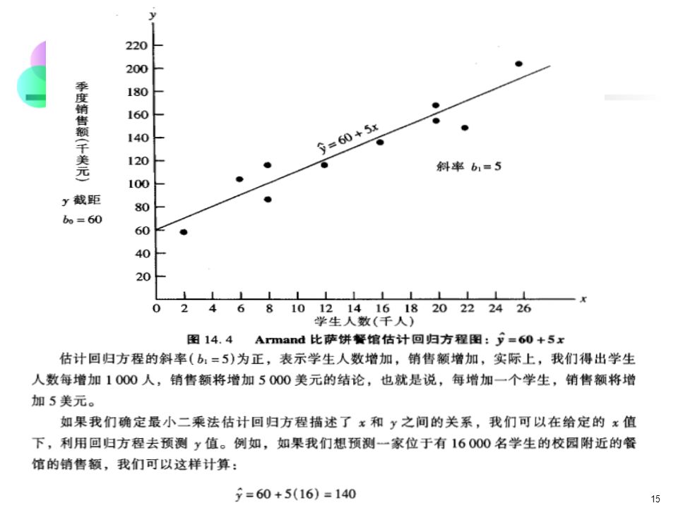
Simple Linear Regression Example

16
Regression Sum of Squares
Measures of Variation Total variation is made up of two parts: SSE 误差平方和 SST 总的平方和 SSR 回归平方和。 Total Sum of Squares Regression Sum of Squares Error Sum of Squares where: = Average value of the dependent variable yi = Observed values of the dependent variable i = Predicted value of y for the given xi value

17
Measures of Variation SST = total sum of squares
(continued) SST = total sum of squares Measures the variation of the yi values around their mean, y SSR = regression sum of squares Explained variation attributable to the linear relationship between x and y SSE = error sum of squares Variation attributable to factors other than the linear relationship between x and y SSE 误差平方和 SST 总的平方和 SSR 回归平方和。利用三者之间的关系来判断估计回归方程的拟合程度。如果应变量都恰巧落在估计回归线上,估计回归方程将给出一个很好的拟合,此时,SSE=0,SSR/SST=1。如果拟合程度差,将会导致SSE变大,SSR/SST变小。
 SST = total sum of squares. Measures the variation of the yi values around their mean, y. SSR = regression sum of squares. Explained variation attributable to the linear relationship between x and y. SSE = error sum of squares. Variation attributable to factors other than the linear relationship between x and y. SSE 误差平方和. SST 总的平方和. SSR 回归平方和。利用三者之间的关系来判断估计回归方程的拟合程度。如果应变量都恰巧落在估计回归线上,估计回归方程将给出一个很好的拟合,此时,SSE=0,SSR/SST=1。如果拟合程度差,将会导致SSE变大,SSR/SST变小。")
18
Measures of Variation _ Y yi _ _ _ y y X y SSE = (yi - yi )2
(continued) Y yi y SSE = (yi - yi )2 _ SST = (yi - y)2 _ y _ SSR = (yi - y)2 _ y y X xi
 Y. yi. y. SSE = (yi - yi )2. _. SST = (yi - y)2. _. y. _. SSR = (yi - y)2. _. y. y. X. xi.")
19
Coefficient of Determination, R2 判定系数
The coefficient of determination is the portion of the total variation in the dependent variable that is explained by variation in the independent variable The coefficient of determination is also called R-squared and is denoted as R2 用估计回归方程来解释总的平方和的百分比 判定系数是判断估计回归方程的拟合程度。然后判定系数越大,那么在没进行适当的模型假设分析之前,就越不能随便使用估计回归方程,判断模型假设是否适当的一个重要步骤是检验关系是否显著。 如果用一个百分比来表示判定系数,R2被解释为用估计回归方程来解释总的平方和的百分比。97.27%的总的平方和能被估计回归方程解释。换句话说,销售收入的变异性有90.27%能被学生人数和销售收入之间的线性关系所解释。 在用最小二乘法估计回归方程和计算相关关系数时,对X和y之间的显著性关系没有进行概率假设和统计检验。R2越大意味着最小二乘法与数据拟合程度越好,也就是说,观察值越靠近最小二乘线。但是如果只有R2,我们不能从统计上得出X和Y之间的关系是显著的结论。这样的结论必须是在考虑了样本容量和最小二乘估计的适当样本分布后得出得。 在实际应用中,的社会科学中遇到得典型数据,R2经常低于0.25,在自然科学和生命科学中得数据,R2经常大于0.6。主要看每个应用的各自特性。 note:

20
Examples of Approximate r2 Values
Y r2 = 1 Perfect linear relationship between X and Y: 100% of the variation in Y is explained by variation in X X r2 = 1 Y X r2 = 1

21
Examples of Approximate r2 Values
Y 0 < r2 < 1 Weaker linear relationships between X and Y: Some but not all of the variation in Y is explained by variation in X X Y X

22
Examples of Approximate r2 Values
Y No linear relationship between X and Y: The value of Y does not depend on X. (None of the variation in Y is explained by variation in X) X r2 = 0
 X. r2 = 0.")
23
Correlation and R2 The coefficient of determination, R2, for a simple regression is equal to the simple correlation squared

24
Estimation of Model Error Variance
An estimator for the variance of the population model error is Division by n – 2 instead of n – 1 is because the simple regression model uses two estimated parameters, b0 and b1, instead of one is called the standard error of the estimate 均方误差(xikemapingfa的估计量)
")
25
Regression Statistics
Excel Output Regression Statistics Multiple R R Square Adjusted R Square Standard Error Observations 10 ANOVA df SS MS F Significance F Regression 1 Residual 8 Total 9 Coefficients t Stat P-value Lower 95% Upper 95% Intercept Square Feet

26
Comparing Standard Errors
se is a measure of the variation of observed y values from the regression line Y Y X X The magnitude of se should always be judged relative to the size of the y values in the sample data i.e., se = $41.33K is moderately small relative to house prices in the $200 - $300K range

27
Inferences About the Regression Model
The variance of the regression slope coefficient (b1) is estimated by where: = Estimate of the standard error of the least squares slope = Standard error of the estimate
 is estimated by. where: = Estimate of the standard error of the least squares slope. = Standard error of the estimate.")
28
Comparing Standard Errors of the Slope
is a measure of the variation in the slope of regression lines from different possible samples Y Y X X

29
Inference about the Slope: t Test
t test for a population slope Is there a linear relationship between X and Y? Null and alternative hypotheses H0: β1 = 0 (no linear relationship) H1: β1 0 (linear relationship does exist) Test statistic 关于显著性检验解释的几点注意:拒绝原假设,得出X和Y之间的关系显著,仍来能得出X和Y之间存在一个因果关系的结论。只有经过分析家从事实上得出这两个变量之间确实存在因果关系,才能认为存在这种因果关系。我们仅仅从统计上得出其显著关系,这种因果关系的结论需要得到理论上的支持,另外需要分析家的准确判断。 拒绝原假设,得出X和Y之间的关系显著,但仍不能得出X和Y之间关系是线性的结论,我们只能得出在X的样本观察值范围内,X和Y是相关的,而且这线性关系是解释Y的变异性的显著部分的结论。 不能把统计显著性与实际显著性混淆。当样本容量很大时,对于小的b1值,我们仍能得出在统计上是显著的结论。而在这种情况下,要得出实际上是显著关系的结论,要特别谨慎。 where: b1 = regression slope coefficient β1 = hypothesized slope sb1 = standard error of the slope
 H1: β1 0 (linear relationship does exist) Test statistic. 关于显著性检验解释的几点注意:拒绝原假设,得出X和Y之间的关系显著,仍来能得出X和Y之间存在一个因果关系的结论。只有经过分析家从事实上得出这两个变量之间确实存在因果关系,才能认为存在这种因果关系。我们仅仅从统计上得出其显著关系,这种因果关系的结论需要得到理论上的支持,另外需要分析家的准确判断。 拒绝原假设,得出X和Y之间的关系显著,但仍不能得出X和Y之间关系是线性的结论,我们只能得出在X的样本观察值范围内,X和Y是相关的,而且这线性关系是解释Y的变异性的显著部分的结论。 不能把统计显著性与实际显著性混淆。当样本容量很大时,对于小的b1值,我们仍能得出在统计上是显著的结论。而在这种情况下,要得出实际上是显著关系的结论,要特别谨慎。 where: b1 = regression slope. coefficient. β1 = hypothesized slope. sb1 = standard. error of the slope.")
30
在线性模型的相关性检验中,如果原假设没有被否定,则表明( )。
(A)两个变量之间没有任何相关关系 (B)两个变量之间不存在显著的线性相关关系 (C)可以排除两变量间存在非线性相关关系 (D)不存在一条曲线能近似地描述两变量间的关系 变量之间的相关程度越低,则相关系数的数值( )。 (A)越小 (B)越接近于0 (C)越接近于-1 (D)越接近于+1
两个变量之间没有任何相关关系. (B)两个变量之间不存在显著的线性相关关系. (C)可以排除两变量间存在非线性相关关系. (D)不存在一条曲线能近似地描述两变量间的关系. 变量之间的相关程度越低,则相关系数的数值( )。 (A)越小 (B)越接近于0 (C)越接近于-1 (D)越接近于+1.")
31
Inference about the Slope: t Test
(continued) Estimated Regression Equation: House Price in $1000s (y) Square Feet (x) 245 1400 312 1600 279 1700 308 1875 199 1100 219 1550 405 2350 324 2450 319 1425 255 The slope of this model is Does square footage of the house affect its sales price?
 Estimated Regression Equation: House Price in $1000s. (y) Square Feet. (x) The slope of this model is Does square footage of the house affect its sales price")
32
Inferences about the Slope: t Test Example
From Excel output: Coefficients Standard Error t Stat P-value Intercept Square Feet t

33
Inferences about the Slope: t Test Example
(continued) Test Statistic: t = 3.329 b1 t H0: β1 = 0 H1: β1 0 From Excel output: Coefficients Standard Error t Stat P-value Intercept Square Feet d.f. = 10-2 = 8 t8,.025 = Decision: Conclusion: Reject H0 a/2=.025 a/2=.025 There is sufficient evidence that square footage affects house price Reject H0 Do not reject H0 Reject H0 -tn-2,α/2 tn-2,α/2 2.3060 3.329
 Test Statistic: t = b1. t. H0: β1 = 0. H1: β1 0. From Excel output: Coefficients. Standard Error. t Stat. P-value. Intercept Square Feet d.f. = 10-2 = 8. t8,.025 = Decision: Conclusion: Reject H0. a/2=.025. a/2=.025. There is sufficient evidence that square footage affects house price. Reject H0. Do not reject H0. Reject H0. -tn-2,α/2. tn-2,α/")
34
Inferences about the Slope: t Test Example
(continued) P-value = P-value H0: β1 = 0 H1: β1 0 From Excel output: Coefficients Standard Error t Stat P-value Intercept Square Feet This is a two-tail test, so the p-value is P(t > 3.329)+P(t < ) = (for 8 d.f.) Decision: P-value < α so Conclusion: Reject H0 There is sufficient evidence that square footage affects house price
 P-value = P-value. H0: β1 = 0. H1: β1 0. From Excel output: Coefficients. Standard Error. t Stat. P-value. Intercept Square Feet This is a two-tail test, so the p-value is. P(t > 3.329)+P(t < ) = (for 8 d.f.) Decision: P-value < α so. Conclusion: Reject H0. There is sufficient evidence that square footage affects house price.")
35
Confidence Interval Estimate for the Slope
Confidence Interval Estimate of the Slope: d.f. = n - 2 Excel Printout for House Prices: Coefficients Standard Error t Stat P-value Lower 95% Upper 95% Intercept Square Feet At 95% level of confidence, the confidence interval for the slope is (0.0337, )
")
36
Confidence Interval Estimate for the Slope
(continued) Coefficients Standard Error t Stat P-value Lower 95% Upper 95% Intercept Square Feet Since the units of the house price variable is $1000s, we are 95% confident that the average impact on sales price is between $33.70 and $ per square foot of house size This 95% confidence interval does not include 0. Conclusion: There is a significant relationship between house price and square feet at the .05 level of significance
 Coefficients. Standard Error. t Stat. P-value. Lower 95% Upper 95% Intercept Square Feet Since the units of the house price variable is $1000s, we are 95% confident that the average impact on sales price is between $33.70 and $ per square foot of house size. This 95% confidence interval does not include 0. Conclusion: There is a significant relationship between house price and square feet at the .05 level of significance.")
37
Prediction The regression equation can be used to predict a value for y, given a particular x For a specified value, xn+1 , the predicted value is

38
Predictions Using Regression Analysis
Predict the price for a house with 2000 square feet: The predicted price for a house with 2000 square feet is ($1,000s) = $317,850
 = $317,850.")
39
Risky to try to extrapolate far beyond the range of observed X’s
Relevant Data Range When using a regression model for prediction, only predict within the relevant range of data Relevant data range Risky to try to extrapolate far beyond the range of observed X’s

40
Estimating Mean Values and Predicting Individual Values
Goal: Form intervals around y to express uncertainty about the value of y for a given xi Confidence Interval for the expected value of y, given xi Y y 区间估计的第一种类型为置信区间估计,是指对于给定的X值,y均值(E(yp))的区间估计。区间估计的第二种类型为预测区间估计,此方法可得出对于给定的x值相对应的y个别值的区间估计。 置信区间和预测区间表示回归结果的正确程度,区间越小表示精确度越高。 y = b0+b1xi Prediction Interval for an single observed y, given xi xi X
)的区间估计。区间估计的第二种类型为预测区间估计,此方法可得出对于给定的x值相对应的y个别值的区间估计。 置信区间和预测区间表示回归结果的正确程度,区间越小表示精确度越高。 y = b0+b1xi. Prediction Interval for an single observed y, given xi. xi. X.")
41
Graphical Analysis The linear regression model is based on minimizing the sum of squared errors If outliers exist, their potentially large squared errors may have a strong influence on the fitted regression line Be sure to examine your data graphically for outliers and extreme points Decide, based on your model and logic, whether the extreme points should remain or be removed

42
Residual Analysis(残差分析)
The residual for observation i, ei, is the difference between its observed and predicted value Check the assumptions of regression by examining the residuals Examine for linearity assumption Examine for constant variance for all levels of X (homoscedasticity,同方差) Evaluate normal distribution assumption Evaluate independence assumption Graphical Analysis of Residuals Can plot residuals vs. X 残差分析是判断模型假定 是否合适的主要模型。
 Evaluate normal distribution assumption. Evaluate independence assumption. Graphical Analysis of Residuals. Can plot residuals vs. X. 残差分析是判断模型假定 是否合适的主要模型。")
43
Residual Analysis 残差提供了有关误差项的最佳信息,因此误差分析是判断误差项的假设是否适当的重要步骤。许多残差分析是基于残差图的观察得出的。 我们利用残差图去验证回归模型假设的有效性,如果验证表明一个或多个假设存在问题,就需要考虑一个不同的回归模型或进行数据转换。 残差分析是用来证实回归模型假设成立的主要方法。即使没有发现任何被违背的假设,也不能得出这个模型给出好的预测的结论。但是,如果有其他的统计检验补充支持显著性结论,并且有较大的确定系数,那么可以用该统计的回归方程得到好的估计值和预测值。

44
Residual Analysis for Linearity
关于x的残差图,是用水平 轴表示自变量的值,用纵轴表示相对应的残差值。 如果对于所有的x值,yipuxunlu的方差都是相同的,并且描述变量之间的回归模型是合理的,那么所有的散点都落在同一条水平带中间。 x x x x residuals residuals Not Linear Linear

45
Residual Analysis for Homoscedasticity
x x x x residuals residuals Constant variance Non-constant variance

46
Residual Analysis for Independence
Not Independent Independent X residuals X residuals X residuals

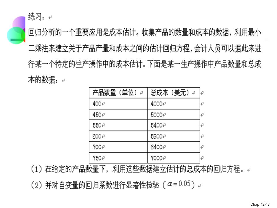
Similar presentations