1. Ch 15 – Inference for Regression

2. Example #1: The following data are pulse rates and heights for a group of 10 female statistics students. Height5559606364 6670 72 Pulse53 5862636568707376 a. Sketch a scatterplot of the data. What is the least-squares regression line for predicting pulse rate from height? where = predicted pulse rates x = height

4. b. What is the correlation coefficient between height and pulse rate? Interpret this number. r = 0.9746 Strong, Positive relationship

5. c. What is the predicted pulse rate of a 59” tall student?

6. d. What is the residual for the 59” student? Height5559606364 6670 72 Pulse53 5862636568707376 53 – 56.54 = – 3.54

7. e. Construct a residual plot and describe its meaning. No pattern, so good linear model

8. Ok, so what is the new stuff for chapter 15? This is not the true line for the population! Where  = true y-intercept and  = true slope of the population

9. Remember: Residuals tell you information about the line and if it is a good model Chapter 15 only focuses on slope. We are going to determine if there is a linear relationship between two variables. (or  = 0)

10. Conditions for Inference: The observations are independent The relationship is linear  Can’t do repeated observations on the same individual!  Look for patterns in the residual plot

11. The standard deviation of the response about the true line is the same everywhere The response varies Normally about the true regression line  Look for spread in the residual plot  Histogram for residuals, look to see if approx normal Conditions for Inference:

12. Standard Error about the LSRL: s = unbiased estimator of  Standard deviation of residuals

13. Calculator Tip!Standard Error Stat – Tests - LinRegTTest L1: x L2: y Use  Leave RegEq blank Calculate s = standard error

14. Confidence Intervals for Regression Slope: where Standard error of the slope

15. SE b estimates the variability in the sampling distribution of the estimated slope (how much slopes vary from experiment to experiment.

16. Minitab Printout: The regression equation is Predicted y = y-intercept + slope  x-variable PredictorCoefStDevTP Constant y-intercept (a)ignoreignoreignore X-variable Slope (b)SEb test-statisticp-value (2-sided) s = standard deviationR-sq = r 2 R-sq(adj) = ignore of residuals

17. Example #1 Infants who cry easily may be more easily stimulated than others. This may be a sign of higher IQ. Child development researchers explored the relationship between the crying of infants four to ten days old and later their IQ test scores. A snap of a rubber band on the sole of the foot caused the infants to cry. The researchers recorded the crying and measured its intensity by the number of peaks in the most active 20 seconds. They later measured the children’s IQ at age three years using the Stanford-Binet IQ test. The data is below.

18. CryingIQCryingIQCryingIQCryingIQ 1087209017941294 1297161001910312103 9 231031310414106 16106271081810910109 18109151121811223113 1511421114161189119 12119121201912016124 20132151332213531135 16136171413015522157 3315913162

19. a. Label all important parts of the Minitab printout. The regression equation is IQ = 91.3 + 1.49 Crycount PredictorCoefStDevTP Constant91.38.93410.220.000 Crycount1.490.48703.070.004 s = 17.50R-sq = 20.7%R-sq(adj) = 21% LSRL (y-int) (slope)(SE b ) (standard deviation of the residuals) (correlation of determination)

20. b. Sketch a scatterplot of the data.

21. c. Calculate the standard deviation of the residuals using your calculator.

22. d. Construct a 95% confidence interval for the slope. P:True slope of the line for crying vs. IQ

23. A: The observations are independent Infants who cry easily may be more easily stimulated than others. This may be a sign of higher IQ. Child development researchers explored the relationship between the crying of infants four to ten days old and later their IQ test scores. A snap of a rubber band on the sole of the foot caused the infants to cry. The researchers recorded the crying and measured its intensity by the number of peaks in the most active 20 seconds. They later measured the children’s IQ at age three years using the Stanford-Binet IQ test. Each infant should be separate from another, not influencing the next test

24. The relationship is linear A: No apparent patterns in the residuals

25. A: The standard deviation of the response about the true line is the same everywhere Residuals spread out evenly

26. The response varies Normally about the true regression line A: Slightly skewed right.

27. Line of regression T-interval N:

28. I: (0.49844, 2.48735)

29. C: I am 95% confident the true slope of the line for crying vs. IQ is between 0.49844 and 2.48735. Note: 0 is not in the interval! This means they have an linear relationship. OR I am 95% confident the mean IQ increases by between 0.49844 and 2.48735 points for each additional peak in crying.

30. Ch 15B – Hypothesis Testing for Slope

31. Remember: so, if r = 0, then b = 0

32. Ho: Or there is no true linear relationship between x and y. Test Statistic:

33. Calculator Tip!Line Regression Test Stat – Tests - LinRegTTest L1: x L2: y Leave RegEq blank

34. Example #1 How well does the number of beers a student drink predict his or her blood alcohol content (BAC). Sixteen students volunteers at Ohio State University drank a randomly assigned number of cans of beer. Thirty minutes later, a police officer measured their BAC. The data is below. Stu #12345678910111213141516 Beer5298373535465714 BAC0.100.030.190.120.040.0950.070.060.020.050.070.100.0850.090.010.05 a. What is the least-squares regression line? where = predicted BAC x = # of beers

35. b. Make a scatterplot of the data and describe its shape. Positive, strong, linear relationship

36. c. What is the correlation coefficient? What does it mean? r = 0.894 Strong, positive relationship

37. d. Label all important parts of the Minitab printout. The regression equation is BAC = – 0.0127 + 0.0180 Beers PredictorCoef StDev TP Constant– 0.0127 0.01264 –1.000.332 Beers0.017964 0.002402 7.480.000 s = 0.02044R-sq = 80%R-sq(adj) = 78.6% LSRL (y-int) (slope) (SE b ) (standard deviation of the residuals) (correlation of determination) (test statistic) (Prob, 2-tailed)

38. e. Verify the results by using your calculator. Stat – Tests - LinRegTTest L1: x L2: y Leave RegEq blank

39. 0.002402

40. f. Conduct the hypothesis test to see if there is a positive relationship between # beers and BAC. P: determine if there is a positive linear relationship between # beers and BAC

41. H: Ho:  =0The number of beers has no effect on BAC Ha:  > 0The number of beers has a positive linear effect on BAC.

42. The relationship is linear A: No apparent patterns in the residuals

43. A: The standard deviation of the response about the true line is the same everywhere Residuals spread out evenly

44. The response varies Normally about the true regression line A:

45. N:Line of Regression T-Test T: 7.48

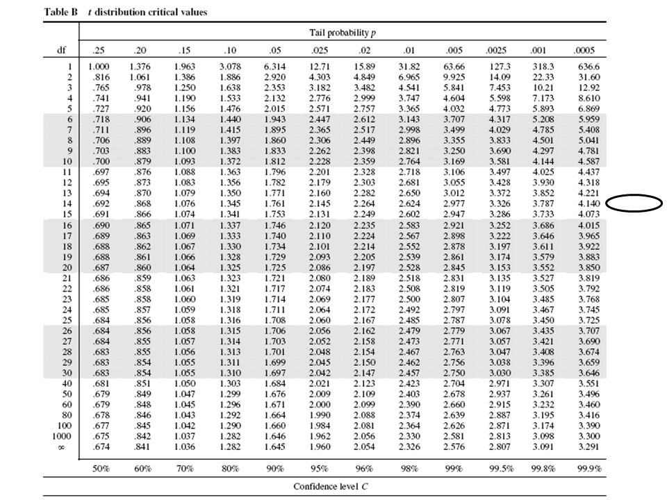
46. O: P(t > 7.48) = df = n – 2 =16 – 2 = 14

48. O: P(t > 7.48) = df = n – 2 =16 – 2 = 14 Less than 0.0005 Or: on calc P(t > 7.48) = 0.000001

49. M: 0.000001 0.05 < Reject the Null

50. S:There is enough evidence to claim that an increased number of beers does increase BAC.