Minnesota AD Model Builder Short Course October 22-24, 2007

Minnesota AD Model Builder Short Course October 22-24, 2007
Thanks to Jim Bence, Brian Linton, and Brian Irwin for providing materials used in previous courses QFC Supporting Partners – MSU, GLFC, Michigan DNR, Minnesota DNR, Ohio DNR, New York DEC, Illinois DNR, Ontario MNR

Quantitative Fisheries Center (QFC)
Created July 2005 Co-directors: Jim Bence and Mike Jones Staffing: Associate Director Computer Programmer Post-Docs (2) Graduate students (3 - PhD; 3 - MS)

Provide research, outreach, and educational services to supporting partners Outreach examples Computer programming support to Michigan DNR inland creel database SCAA consultation for Lake Erie percid assessments River classifications in MI, WI, NY, PA Power analysis for OhDNR Lake Erie gill net surveys

Education AD Model Builder short courses taught in East Lansing (2006, 2007) and Cornell Biological Field Station (2007) Online Maximum Likelihood Estimation course (launched October 16, 2007) Introduction to R short course (currently being converted to an online format) Online Resampling Approaches to Data Analysis course (planned for summer 2008)

How this course will differ from previous offerings
More emphasis on straightforward applications More hands on programming (coding the whole program rather than only bits and pieces) Less emphasis on coding efficiency (comes with practice) Limit the number of new concepts – new model, new software, new to programming = disaster Tell students that corrected versions of the code and this presentation will be available over the internet within a couple of weeks

What is AD Model Builder and why should you use it?
Auto Differentiation Model Builder Software for creating computer programs to estimate parameters of statistical models

What are the advantages of using it?
Fast and accurate Flexible Designed for general maximum likelihood problems Libraries for Bayesian and robust estimation methods Includes many advanced programming options (estimation in phases) Multi-dimensional arrays

How fast is it? Evaluation by Schnute and Olsen
100 parameter catch-at-age model from Schnute and Richards (2005) Package msec/ Function call Number of function calls Time to converge ADMB 131 291 38 seconds Gauss 167 23,365 1.08 hours Matlab 639 18,360 3.25 hours S-plus n/a

Why is it so fast? Auto differentiation – a method for approximating derivatives to within numerical precision Most other computer programs actually calculate derivatives with respect to every parameter (finite differences) Newton-Raphson – requires first and second order derivatives Levenberg-Marquardt – requires first order derivatives

What are some of the most noticeable differences with other software packages?
Users must specify the objective function to be minimized (Note: ADMB only does minimization)

Objective function Parameter value
Definition of objective function – a function that defines how well your data fit a particular hypothesis (e.g., sum of square errors, sum of absolute errors, likelihood)

ADMB Differences with SAS
data lenweight; input length weight; datalines; . 12542 15909 ; Run;

proc nlin data=lenweight; parameters a=0 b=3; model weight=a*length**b; run; Proc NLIN estimates parameters by (weighted) least squares; minimize the sum of square errors

proc nlmixed data=lenweight; ypred=alpha*length**beta; parms alpha=0.001, beta=3, sigma=1; model weight~normal(ypred,sigma); run; Proc NLMIXED estimates parameters by maximum likelihood

proc nlp data=lenweight tech=newrap inest=par1 outest=opar1 maxiter=1000; parms a, b, sigma; ypred=a*Length**b; nlogl = log(sigma)+0.5*((weight-ypred)/sigma)**2; min nlogl; run; Proc NLP (NonLinear Programming) in SAS/OR is an estimation method similar in vein to that of ADMB in that analysts must specify their objective function

What are the most striking differences with other packages?
Users specify the objective function to be minimized Steps to running Create an ADMB template Convert template to C++ code Compile – convert from programming code to machine code (creates an executable file) Link the executable file to C++ libraries Run your executable file Resulting executable can be run on similar datasets on any computer

What are the difficulties associated with using ADMB?
Requires a more intimate knowledge of statistical theory (probability distributions, likelihoods, Hessians) Some knowledge of C++ is required Code can be a little quirky (as you will soon see) Also, less than stellar help manuals

ADMB Files Input Output .tpl – make the model .dat – input data
.pin – initial values (optional; need to specify for all parameters) Output .par – parameters estimates .cor – correlation of parameters .std – parameter estimates with std. deviations .rep – user-defined outputs (optional)

ADMB Files Input Output
ADMB will expect .dat and .pin files to have same name as .tpl e.g., MilleLacs.tpl, MilleLacs.dat (this can be overridden) Output By default, output files will have same file name e.g., MilleLacs.rep, MilleLacs.par (this can be overridden) Note: In the project folder, ignore the files with the extra ~ on the extension… e.g., Oneida.tpl~ they are temporary files (so be sure you open the right file).

.dat file Simply contains the data you will use when fitting your model Simple.dat #Simple linear regression example #For ADMB Short Course 1, August 2007 #Created by D. Fournier, modified by B. Linton #Any text after "#" is ignored # number of observations 10 # observed Y values # observed x values Note: no column headers, no semicolons, - Could be a single line of data if you wanted

.tpl Sections DATA_SECTION PARAMETER_SECTION INITIALIZATION_SECTION
PROCEDURE_SECTION Each must be written just like that REPORT_SECTION Other commonly used section PRELIMINARY_CALCS_SECTION LOCAL_CALCS

Keep in mind Different sections use different programming languages
Data, Parameter, Initialization sections used ADMB code Procedure, Report, Local Calcs, Preliminary Calcs sections use C++ code Lines typically must end with ; Not absolute as in SAS (loops, conditional statements) You can use C++ code in the Data, parameter, and initialization sections but you must tell AD Model Builder that you are doing this

Keep in mind Comments in .dat file are specified with ‘#”
Comments in .tpl are specified with ‘//’ You can use C++ code in the Data, parameter, and initialization sections but you must tell AD Model Builder that you are doing this

Keep in mind Section heads (DATA_SECTION, PARAMETER_SECTION) must be left justified Except LOCAL_CALCS section, requires one space before typing LOCAL_CALCS All other lines should have two spaces before the text

.tpl Sections DATA_SECTION
Identify values that will be read-in from .dat file Need to consider the order of numbers in your .dat file Can read your data in as integers, real numbers, matrices, arrays,… DATA_SECTION init_int first_year init_int last_year init_int first_age init_int last_age init_number lambda init_matrix obs_length(first_year,last_year,first_age,last_age) Note the two spaces Obs_length – years are the rows of the matrix, ages are the matrix columns

Also where you can declare your looping variable; valid throughout your entire code DATA_SECTION init_int first_year init_int last_year init_int first_age init_int last_age init_number lambda init_matrix obs_length(first_year,last_year,first_age,last_age) int i int j Obs_length – years are the rows, ages are the columns Because i and j are missing init in front of them, nothing is read in from the .dat file – you are simply declaring it as a variable that you will use; similar to VBA programming

If .dat doesn’t have the same name as .tpl
.tpl Sections DATA_SECTION If .dat doesn’t have the same name as .tpl Assume program is MyModel.tpl Then, default search is for MyModel.dat Code below will read-in a file named ControlFile.dat: !!ad_comm::change_datafile_name("ControlFile.dat"); Can also go back: !!ad_comm::change_datafile_name(“MyModel.dat"); !! – tells ADMB that what follows is C++ code !! Indicates that what follows is c++ code

.tpl Sections DATA_SECTION Always a good idea to verify that your data have been read in correctly In .dat file, have as your last entry In Data_section, specify init_int test as the last read in variable and type !!cout << test << endl; !!exit(99); !! Indicates that what follows is c++ code

DATA_SECTION //Read data in from simple.dat init_int nobs //number of observations init_vector Y(1,nobs) //observed Y values init_vector x(1,nobs) //observed x values init_int test //test variable !!cout << test << endl; !!exit(99); !! Indicates that what follows is c++ code When you run your executable, the program will write out the test number and then stop; doesn’t execute the entire thing

.tpl Sections DATA_SECTION PARAMETER_SECTION
Define Parameters – the values to be estimated (must have at least 1) use loge scale, if only interested in non-negative parameter space Identified by the prefix init_ Intermediary Variables - quantities that will change as a result of parameter estimation Can also declare index variables here. Also, if “containers” are needed just for output and not for calculations, then put those here too. Name your Objective Function – the quantity to be minimized

.tpl Sections DATA_SECTION PARAMETER_SECTION PARAMETER_SECTION
//Parameters to be estimated init_number a //slope parameter init_number b //intercept parameter //Quantities calculated from parameters vector pred_Y(1,nobs) //predicted Y values //Value to be minimized by ADMB objective_function_value rss //residual sum of squares objective_function_value must be specified

Keep in mind Init_ in DATA_SECTION indicates a value that will be read in from the .dat file Init_ in PARAMETER_SECTION specifies a variable that will be estimated

Set Initial values for parameters - use in place of .pin file log_F -1.0 log_M -1.6 You should always assign a starting value – default starting value in ADMB is 0 If you are using a bounded variable, the starting value is halfway between the upper and lower bound

PROCEDURE_SECTION Back transform parameters for use in functions (if needed) e.g., F = exp(log_F) Construct Functions Specify the equation for your Objective function Must have a PROCEDURE_SECTION for model to compile

.tpl Sections PROCEDURE_SECTION DATA_SECTION
init_int nobs //number of observations init_vector Y(1,nobs) //observed Y values init_vector x(1,nobs) //observed x values PARAMETER_SECTION init_number a //slope parameter init_number b //intercept parameter vector pred_Y(1,nobs) //predicted Y values objective_function_value rss //residual sum of squares PROCEDURE_SECTION //Simple linear model gives predicted Y values pred_Y=a*x+b; //Parameter estimates obtained by minimizing //objective function value (residual sum of squares) rss=norm2(Y-pred_Y); //norm2(x)=x1^2+x2^2+...+xn^2

PROCEDURE_SECTION REPORT_SECTION Specify output to go to .rep file Be sure to end .tpl with an empty line (hard return)

.tpl Sections Report section useful for reporting values not otherwise needed in the model Can be organized in many ways Can still do calculations in REPORT_SECTION e.g., report<< “S: ” << exp(-Z) <<endl; Results (.rep file) can be read into other programs

Create an Output .dat file
Append to file Use an output file stream ofstream ofs(“MyOutput.dat”,ios::app); { ofs << “Output variable x: “ << x << endl; ofs << “Output variable y: “ << y << endl; } Also can delete a file system(“del MyOutput.dat); Note: different system command for Linux

Other .tpl Sections PRELIMINARY_CALCS_SECTION Uses C++ code
Can do some preliminary calculations and manipulations with the data before getting into the model proper e.g., pi = 3.14; RUNTIME_SECTION Change behavior of function minimizer TOP_OF_MAIN_SECTION Change AUTODIFF global variables

Compare with SAS code Data Section Runtime Section
DATA GROWTH; INPUT AGE LENGTH GENDER; DATALINES; PROC NLIN DATA=GROWTH METHOD=MARQUARDT; PARAMETERS LINF1 = 1100 K1=0.4 T01=0.0; YPRED= LINF1*(1-EXP(-K1*(AGE-T01))); MODEL LENGTH = YPRED; OUTPUT OUT=DATA_OUT PRED=PP RES=RR; RUN; Data Section Runtime Section Initialization Section Prelim Calcs Section Procedure Section Report Section

.tpl File General rule: make .tpl file as general as possible (try to avoid hard coding) – will allow you to analyze future datasets Must be “compiled” into C++ code 1) tpl2cpp (makes .cpp file) 2) compile (makes .exe file) 3) link (connects libraries) We’ll use Emacs (more later)

Compiling your .tpl Need a C++ compiler to run your code
After it is compiled, model will be a .exe (so can be run on machines without ADMB) If you change the .tpl file, it must be recompiled… If you change and save data (values, sometimes dimensions), the existing model will still be ready to go… So, advantage to putting starting values, ect…, into .dat or .pin files.

How should I build my tpl
Suggestions Keep projects in separate folder Name, describe, and date each file at the top Start with a simple working program Be sure data get read in correctly Use unique names for files and parameters (don’t use “catch” as a variable name) Avoid “hard coding” … make it flexible Build it one step at a time COMMENT, COMMENT, COMMENT

About Emacs For this class, you will Emacs to construct your .tpl file
A highly customizable text editor We have modified Emacs so that an ADMB .tpl file is automatically linked to a C++ compiler MINGW32 is a freeware C++ compiler – don’t need to buy both ADMB and Visual Studio

Using Emacs Refer to Emacs Basics handout Hotkeys are different
e.g., “control-v” will not paste Highlighting text will automatically copy it Remember to save files and recompile .tpl

Let’s Try an Example Simple linear regression model
Estimation by least squares

Let’s Try an Example Start Emacs by double clicking the Emacs icon on the desktop Things to show students How to create a file Split window Copy and paste Practice some of the hot key functions Open the tpl

Let’s Try an Example Open the simple.tpl and simple.dat files in the MNADMB folder located on your desktop Things to show students The different menuiing system that opens up when a .tpl file is active Review the steps in converting a tpl file to an executable file Open the .cpp file that results Safe mode – automates all the above steps while still outputting the results from the different parts Non-safe mode – automates the steps, won’t tell you if an error occurs Run –est – suppressed calculation of the standard errors of the parameters Run… switch Explain the norm2 command Have them open the .par, .std, and .cor files with notepad Have them add in an INITIALIZATION_SECTION and REPORT_SECTION Report out residuals and r-square value, better estimate of sigma Show the importance of verifying data read in correctly – run simple_dummy1 tpl Various ways of using cout commands (data section, local_calcs, preliminary_calcs_section Show them how they can copy their executable and run it on a different dataset Add the command cout << a << " " << b << " " << rss << endl; To the end of the procedure section to show parameter search

Illustrates the parameter search for the Intercept witn starting value of 0 and the change in the objective function

Would never do this. Analytical solutions available for simple linear regression. Numerical search is overkill.

Simple Diagnostics Types of error messages: Modes of operation:
Compile Run-time Modes of operation: Safe mode Optimization mode

Compile Errors Error in line 48 while reading r
Line number refers to tpl file Need a space at start of each line of code Except for comments and section headings Need a “return” after last line of tpl

Compile Errors c:/…/simple.cpp:36: error: expected `;' before "rss“
c:/…/simple.cpp:35: error: `pred_Y' undeclared (first use this function) Check designated line in cpp file Make corrections to tpl file, not cpp file

Run-Time Errors Error reading in dat file – no error message
In DATA_SECTION, values made up for init_objects that are not assigned values from dat file Use “cout” command to make sure dat file reads in properly

Run-Time Errors IND0: infinity or division by zero
Var Value Gradient #IND0e+000 #QNANe+000 IND0: infinity or division by zero QNAN: not a real number Use “cout” command to check calculations

Run-Time Errors Error in matrix inverse -- matrix singular in inv(dmatrix) Hessian cannot be inverted to obtain asymptotic standard errors Use different parameter starting values Reparameterize model

Run-Time Errors array bound exceeded -- index too high in prevariable::operator[] Tried to assign value outside the defined range indices for vector or matrix Define a vector to be 10 elements long Write values to the vector using a loop with 11 steps Use “cout” command to locate error in tpl Error message only appears when in safe mode

Modes of Operation Safe mode: provides bounds checking on all array objects ADModel > tpl2cpp > compile > link ADModel > makeadms Optimization mode: provides faster execution ADModel > makeadm Note, little difference in speed unless you have a very complex model

Essential theory

Goal – Model Building Models are tools for evaluating hypotheses
Uses of models Improved understanding of a system Prediction Help in making decisions Likely to have several competing models that you will want to fit and compare Many different types of estimation procedures to consider – we will consider maximum likelihood

Additional Information
Online MLE Course Launched 16 Oct. 2007 Registration at Normal Cost: $370 to QFC Supporting Partners $300 if you contact me by November 5

Background on maximum likelihood
Likelihood – a measure of how likely a set of parameters are to have produced your data Can be confusing. Often written as: But not always – Think of as function of parameters. Depends upon data. Likelihoods are mathematically the same as probability distributions; thus, you must consider what probability distribution gave rise to your data

Probability density functions
Functions describing the probability of obtaining a particular outcome for a random variable For discrete distributions, sometimes referred to as probability mass functions Typically denoted as (x) or as (x|θ)

Properties of probability distributions
Probability density functions (pdf) for continuous distributions Probability mass functions (pmf) for discrete distributions Joint pdf/pmf for multiple independent observations

A familiar example A single observation from a normal distribution
Probability density function

The likelihood function
Mathematically equal to the joint probability density function But NOT a probability density for parameters Maximum likelihood estimates are values of parameters that maximize the likelihood

Properties of maximum likelihood estimates
Invariant to transformations Asymptotically efficient (lowest possible variance) Asymptotically normally distributed Asymptotically unbiased (expected value of the estimated parameter equals the true value) If we assume independent, normally distributed errors, ML methods provide the same estimates of structural parameters as least squares. E.g., can be biased for small n Summary – versatile and widely used with a number of desirable properties, but not perfect! For normal distribution

Back to really, really, really simple example: Normal, one observation, variance known
Likelihood equal to the probability density function x = 12 Maximum likelihood estimates are values of parameters that maximize the likelihood

Slightly more complicated example – normal sample (multiple observations)

To ease calculations, typically take the negative log of the likelihood
Parameter estimates that maximum the likelihood are the same values that will minimize the negative log likelihood

Slightly more complicated example – regression

Ignoring constants If you minimize negative log likelihood you can ignore constants because: For same q will minimize left and right hand side Example of the reduced (ignored constants dropped) negative log likelihood (for normal). This depends on what you estimate.

Concentrated Likelihood
Reduce the number of parameters by writing some parameters as a function of other parameters

Concentrated Likelihood

Combining normal data with different variances
Data are: {y11, y12, …y1k1, y21, y22, …y2k2} Plus known predictors X First and second set of y have different distributions (variances) -logL= L1+L2+IC: Just special case of rule for getting joint pdf for independent data

Concentrated negative log likelihood when there is more than one normal component
Lambda’s are a weighting factor – how strong a role should a particular data set play in influencing the overall fit of the model

Likelihood for Lognormal Distribution

Von Bertalanffy Growth Model
Welcome to nonlinearity

Example – Modeling size versus age

Von Bertalanffy Model

Let’s write some code….. Check out your .dat file (number of observations, data for individual fish, dummy variable) Start out by reading in your data Use the simple.tpl as an example Use the concentrated likelihood for the normal distribution as your obj. function Initial values – Linf=1200 mm, t0 = 0, Growth coefficient = 0.4

Hints Read age and length data in as a matrix
e.g., init_matrix fish(1,nobs,1,2) Create an age and length vector e.g., vector ages(1,nobs) Extract age and length data from the matrix using the extract column command (column) e.g. ages = column(fish,1)

Let’s write some code….. Advanced things to try
Linf and Kappa must be positive so try estimating on a log scale Use the full negative log likelihood as your objective function (sigma will be another parameter that will need to be estimated; also will need to be estimated on a log scale)

Mortality estimation Tag-recovery studies widely used to estimate fishing and natural mortality rates Expected number of tag recaptures generally considered to follow a multinomial distribution

Mortality model Expected number of tag recaptures generally considered to follow a multinomial distribution

Mortality model Expected numbers of recaptures Recovery Periods
Year marked # Marked 1 2 3 4 N1 N1f1 N1S1f2 N1S1S2f3 N1S1S2S3f4 N2 N2f2 N2S2f3 N2S2S3f4 N3 N3f3 N3S3f4 K=4 N4 N4f4 S = probability a fish survives the year f = probability a fish is harvested by angler and its tag is retrieved and reported

Instantaneous mortality formulation
Prob. surviving previous time periods Prob. harvest during time period

Let’s write some code….. Estimate Fs and Ms on the log scale
Assume =0.18 for all years Use report section to calculate instantaneous total mortality for each year Use report section to calculate exploitation rate

Advanced things to try…..
Create an output vector of predicted tag recoveries to see how well model agrees with observed data Try different objective functions and see how results match with one another

Day 2 Questions before proceeding???

Strategy for building your tpl from scratch
Start with a working file from another problem, as memory aid on coding syntax etc (section names, define variables, loops…). First create a minimal program which consists of the required data, parameter, and procedure sections, has an objective function variable and one estimable parameter. Check that the program reads the data in correctly (use cout and exit)

Strategy for building your tpl from scratch
Sequentially add calculations to the procedure section and check they work using cout and exit. Much easier to check things as you build them up rather than trying to find where the errors are after writing lots of code. Use small steps and do not worry about efficiency too much at this stage. Make sure the estimation procedure is working before investing time in defining derived variables in report section.

Quick Refresher In LN_Density folder is a dataset that was generated by random draw from a lognormal density (μ = 10, σ2 = 1.5) Use ADMB to find MLEs of μ and σ2

Alewife stock recruitment in Lake Huron
What effect would reduction in salmonid stocking by OMNR and MiDNR have on fish communities? Stock-recruitment relationships of prey species (alewife, rainbow smelt) recognized as major source of uncertainty

Alewife spawners vs. recruits

Ricker stock-recruitment curve
Additive Error Multiplicative Error If X~N(μ,σ2) and Y = exp(X) then Y~LN(μ,σ2)

Linearized form of multiplicative error To calculate R/S use the elem_div(x,y) command To calculate R/S when R and S are vectors, use the command elem_div(R,S). Don’t forget to declare a vector where your predicted values will go

Linearized form

Things to try….. Estimate the linearized version of the multiplicative error form of the recruitment model Estimate the additive error form of the recruitment model (try using concentrated likelihood)

Inference using AD Model Builder

An overview on inference
By inference, I mean going beyond point estimates and saying something about the quality of the estimates. How likely is it that the estimate is close to the true value? Topics related to inference Estimates of standard errors Confidence intervals Bayesian probability intervals

Inferences depend upon the variance-covariance matrix: Diagonal elements are variances of parameter estimates, off-diagonals are covariances among parameter estimates.

What is a variance and covariance?
Recall definition of expected value

Covariances and parameter estimates
The variances describe uncertainty in the parameter estimates. The square-root of the variances gives the standard errors The covariances describe how the estimation errors for two parameters are related. When parameter “a” is over-estimated does parameter “b” also tend to be over-estimated (+ cov), tend to be under-estimated (- cov) or is there no relationship (0 cov)?

Correlation matrix Diagonals are 1.0
Off diagonals are correlations among parameter estimates:

Asymptotic results for parameters
Done automatically in ADMB (i.e., you don’t have to code anything) Results are in *.std and *.cor These are based on the Hessian matrix: Hessian – matrix of second-order partial derivatives of the likelihood with respect to the parameters

measures how likelihood falls off away from best estimate

Cross derivatives “twist” the likelihood surface
Cross derivatives “twist” the likelihood surface. Not counting for them would cause underestimation of uncertainty!

index name value std dev
Example *.std output index name value std dev 1 log_q e e+000 2 log_popscale e e-001 3 log_sel_par e e+000 4 log_sel_par e e+000 5 log_sel_par e e+000 6 log_sel_par e e+000 7 log_sel_par e e+000 8 log_sel_par e e+000 9 log_relpop e e-001 10 log_relpop e e-001 11 log_relpop e e-001 … … … …

Example of *.cor file index name value std dev 1 2 3 4 5
1 log_q e e 2 log_popscale e e 3 log_sel_par e e 4 log_sel_par e e 5 log_sel_par e e 6 log_sel_pa ….. … … … … … … … … … … … … … … … … … …

What happens if we use RSS instead of neg logL or neg logConc?
Made this change to growth.tpl // conc=(nobs/2.0)*log(rss); //concentrated likelihood //changed obj function to just be RSS for illustrative purposes //DO NOT DO THIS conc=rss; Note that these are results from a different dataset then what they are using; point is still the same

Standard errors for derived quantities
Often we are interested in assessing the uncertainty of derived quantities (quantities that are functions of one or model parameters) biomass in last year of assessment, MSY for a logistic surplus production model, ratio of abundance in 2002 to abundance in 1995, SSBR based on recent mortality schedule,… Calculated using the Delta method

Delta method Method for approximating statistical properties of nonlinear functions of random variables based on a Taylor series approximation of a function Second order Taylor series expansion of g(theta)

Delta method Method for approximating statistical properties of nonlinear functions of random variables based on a Taylor series approximation of a function First order Taylor series expansion of g(theta)

Delta method For functions of several random variables, method requires partial derivatives, covariances, … Approximation of variances less accurate then approximations of expectations (first versus second order Taylor series expansion) Also used to estimate standard errors of derived quantities in SAS (Proc NLMIXED, PROC GLIMMIX)

Standard error estimates for derived quantities (continued)
Can be done for any type of variable (number, vector, matrix) Specified in PARAMETER_SECTION sdreport_number Z sdreport_vector predicted_N (2,nages) Results are included in *.std and *.cor files

Refer to simple.tpl

Asymptotic standard errors can produce misleading inferences
When sample sizes are small The curvature of the likelihood surface changes substantially within the range of plausible estimates – i.e., “near to the maximum likelihood estimates

Profile Likelihood Method
Typically, a method for constructing confidence intervals where analysts vary one or more parameters systematically and computes the values of the other parameters that maximize the likelihood Surface of the likelihood used to construct confidence intervals based on a chi-square distribution

Profile Likelihood Method (cont.)
Construct profile likelihood for growth coefficient of von Bertalanffy growth model (MLE = 0.281) Kappa (fixed) L (estimated) -logL -2.0 SE = 0.11 34.19 2.45 -1.0 SE = 0.18 29.04 1.88 -0.5 SE = 0.22 27.22 1.64 +0.5 SE = 0.35 24.58 1.68 +1.0 SE = 0.44 23.66 2.15 +2.0 SE = 0.58 22.33 3.97

Profile Likelihood Method (cont.)

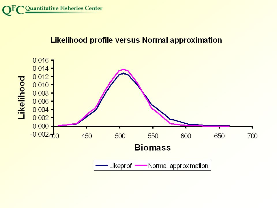
Profile Likelihood Method
This is NOT inverting a likelihood ratio test in ADMB land! This is Bayesian in philosophy (in the same way that MCMC is). Can also be motivated by likelihood theory (support intervals) Idea is to use the profile for g() to approximate the probability density function for g.

How to use the profile method
Declare a variable you would like to profile as type likeprof_number in the parameter section, and assign it the correct value in the procedure section. When you run your program use the lprof switch: run -lprof Results are saved in xxxxx.plt where xxxxx is the name of your likeprof_number variable Your variable is varied over a “profile” of values and the best fit constrained to match each value of your variable is found

PLT File contains list of point (x,y) x is value (say biomass)
y is associated prob density Plot of Y vs X gives picture of prob distribution ADMB manual says estimate probability x in (xr,xs) by The sum from r to s is over intervals of x longer than the interval of interest. If all intervals same length (they seem to generally be)d, then it is d too long. An alternative would be to drop the sth term from the sum, but then the prob really would be for r-d/2 to s-d/2. If the length of the intervals were not constant then it would be better to use (xi+1 - xi-1)/2 * yi in the sum and the end points would depend upon width of intervals at the ends.

Profile likelihood options
Switch -prsave This saves the parameter values associated with each step of profile in myvar.pv Options set in tpl (preliminary calcs section): e.g., for lprof var myvar: PRELIMINARY_CALCS_SECTION myvar.set_stepnumber(10); // default is 8 myvar.set_stepsize(0.2); //default is 0.5 Note manuals says stepsize is in estimated standard deviations but this appears to be altered adaptively during the profile WARNING -- LOTS OF STEPS CAN TAKE LOTS OF TIME!

Exercises Calculate asymptotic standard errors and likelihood profiles for Growth model – parameters of growth model; predictions of length at age (asymptotic only) Mortality model – Z=M+F and u=FA/Z Stock recruitment model (linear version of the multiplicative error) RMax is the maximum level of recruitment Mu msy is the optimum harvest rate for MSY Remember, with linear version and simple linear regression, β0 estimates log and β1 estimates β

Essential Programming Skills
New ADMB concepts and techniques Loops Conditional statements Bounded objects User-defined functions Random number generation

Loops Repeats code a specified number of times for (i=m;i<=n;i++) {
; } for (i=10, i>=0, i-=2) looping variable ‘i’ goes from ‘m’ to ‘n’ in increments of 1 Code that is repeated for each increment of ‘i’ Note that there is no semicolon for the for line or the parentheses ‘i’ goes from 10 to 0 in increments of -2

Refer to loop.tpl

Conditional Statements
Runs code if conditions met if (condition) { ; } if condition is true then run this code Again, note that there is no parentheses on the if line or the line for parentheses

Common Conditional Statements
(X==Y) X equal to Y (X!=Y) X not equal to Y (X<Y) X less than Y (X<=Y) X less than or equal to Y (X>Y) X greater than Y (X>=Y) X greater than or equal to Y Use && for compound statements e.g., if (iyear=1998 && iarea=north) Use || for or statement e.g., if (iyear=1998 || iyear=2000)

Conditional Statements
if (condition) { ; } else if condition is true then run this code if condition is false then run this code

Advanced Conditional Statements
active(parameter) Returns true if parameter is being estimated last_phase() Returns true if in last phase of estimation mceval_phase() Returns true if –mceval switch is used sd_phase() Returns true if in SD report phase

Refer to conditional.tpl

Bounded Objects Bounds constrain what values a parameter can take
init_bounded_number x(-10,10) init_bounded_vector y(1,nobs,-10,10) Lower bound Upper bound Bounding parameters useful for keeping the objective function away from flat areas; can be used to specify uniform priors for parameters in Bayesian analysis

User-Defined Functions
Organize code in PROCEDURE_SECTION function_name(); FUNCTION function_name ; Call function for use Define function Notice that no parentheses are used in the definition of the function, but they are needed to call the function Call function for use Build function Code for function

Functions that take arguments
Functions that do not take arguments can be used to organize code get_catch_at_age(); Functions that take arguments can simplify calculations rss=norm2(residuals); Beware of functions that take parameters as arguments

Refer to function.tpl

Random Number Generator
Initialize random number generator (x) random_number_generator x(seed); Fill object (y) with random numbers y.fill_randn(x); // yi~Normal(0,1) y.fill_randu(x); //yi~Uniform(0,1) Random number seed

Random Number Generator
Random number generator produces pseudo-random numbers Pseudo-random numbers are generated from an algorithm which is a function of the random number seed The same random number seed will always produce the same string of numbers

Exercises Modify the growth.tpl so that you use a loop rather than the norm2 command to calculate the residual sum of squares

Now to code it…

Piecewise regression catch curve
Maceina (2007) recently proposed using piecewise regression to estimate size related mortality rates by catch curves

Knot or joinpoint

4 parameters (β0, β1, β2, knot) [actually 5 with 1 linear constraint] Knot should be initialized as a bounded variable (minimum and maximum age) Use a loop and conditional statement to estimate predicted ln catch at age for different fish ages Use concentrated log likelihood (assume normal)

Caveat This estimation approach is similar to the one taken in Maceina (2007) However, this is not the generally recommended approach for piecewise models Grid search recommended Search for regression parameters across a grid of knots Fix the knot, estimate the regression parameters

Now to code it…

Convergence Issues Convergence criteria
Diagnosing convergence problems Convergence messages Self diagnostics Fixing convergence problems Convergence criteria problems Code problems

Convergence Criteria Gradients close to zero
Maximum |gradient| < 1x10-4 Obj. function value fails to decrease Change < 1x10-6 for 10 iterations in a row Obj. function evaluated too many times Maximum evaluations = 1,000 Line search fails to find parameters with lower objective function value Step size adjusted 30 times

Convergence Messages Run-time messages indicating convergence problems
ic > imax in fminim is answer attained ? Function minimizer not making progress ... is minimum attained? Minimprove criterion = e+000 Run-time messages indicating convergence problems

Self Diagnostics Compare smallest and largest eigenvalues of Hessian in eva file Is logarithm of determinant of Hessian small in cor file? Are correlations large in cor file? Are standard errors large compared to parameter value in std file? Examine trajectory of iterations including objective function and key parameters

Convergence Criteria Problems
Is convergence criteria too strict or too loose? Does objective function value change substantially as gradients approach convergence criterion? Are results sensitive to changes in convergence criterion? Try different parameter starting values

Changing Convergence Criteria
In tpl file RUNTIME_SECTION convergence_criteria 0.001 maximum_function_evaluations 500 With runtime switches -crit –maxfn 500 Switch to restart (after rescaling) if function not improving but gradients not near zero -rs

Code Problems Do predictions respond to parameter values?
If not possible can estimate parameters in different phases Parameterize the current function differently Or use a different function

Improving Efficiency You do not need to worry about model efficiency in most cases In general, it is only important when: Your model is very complex You are running your model many times (e.g., mcmc, simulation study)

Efficiency rule number 1 – calculate something only once if you can!
Quantities that do not change but are needed during estimation should be calculated in PRELIMINARY_CALCS_SECTION Quantities that are not needed for estimation but only for reporting should be calculated in REPORT_SECTION or if uncertainty estimates are needed conditional on phase too: If (sd_phase()) {… }

Efficiency rule number 2 – avoid unneeded loops
Use admb built in functions (e.g., sum, rowsum, element by element multiplication and division, etc) Combine loops over the same index

Bayesian Inference in AD Model Builder
Bayesian inference – a different philosophical approach to statistics than traditional inference Essential element is the use of observed data to transform numerical estimates of our degree of belief in a hypothesis into posterior distributions that take into account the evidence in the observed data

Bayesian Inference ADMB presumes we are going to start by finding the parameters that maximize the posterior density (called highest posterior or modal estimates), so just minimize the log posterior. Just like a negative log-likelihood but with new terms for priors

Markov Chain Monte Carlo
Calculation of posterior distributions can be mathematically intractable accept for trivial scenarios Markov Chain Monte Carlo method is an algorithmic way to generate samples from a complex multivariate pdf (in practice, usually the posterior distribution). This is useful in looking at marginal distributions of derived quantities. These marginal distributions are the same thing the profile likelihood method was approximating.

Specifying Priors If prior on M were log-normal with median of 0.2 and with sd for ln(M)=0.1, then just add to your likelihood: For special case of diffuse prior ln(p()) is constant inside the bounds, so a bounded diffuse prior can be specified just by setting bounds on parameters.

Doing an MCMC run Use -mcmc N switch to generate a chain of length N. Default N is 100,000. Summarized output for parameters, sdreport variables and likeprof_numbers is in *.hst This automatic summary is for the entire chain with no provision for discarding a burn-in and no built in diagnostics. Serious evaluation of the validity of the MCMC results requires you gain access to the chain values.

Gaining access to chain values
When you do the MCMC run, add the switch -mcsave N, which saves in a binary file every Nth values from the chain. You can rerun your program to read in the saved results and make one run through your model for each saved set of parameters. Use the switch -mceval You can add code to your program to write out results (and do special calculations) during the mceval phase. You can modify your program to do this even after you generate your chain, provided your change does influence the posterior density.

Example of code to write results out when using mceval switch
if (mceval_phase()) cout << Blast << endl; Important caution: this writes to standard output. Better redirect this to file or millions or numbers will go scrolling by!

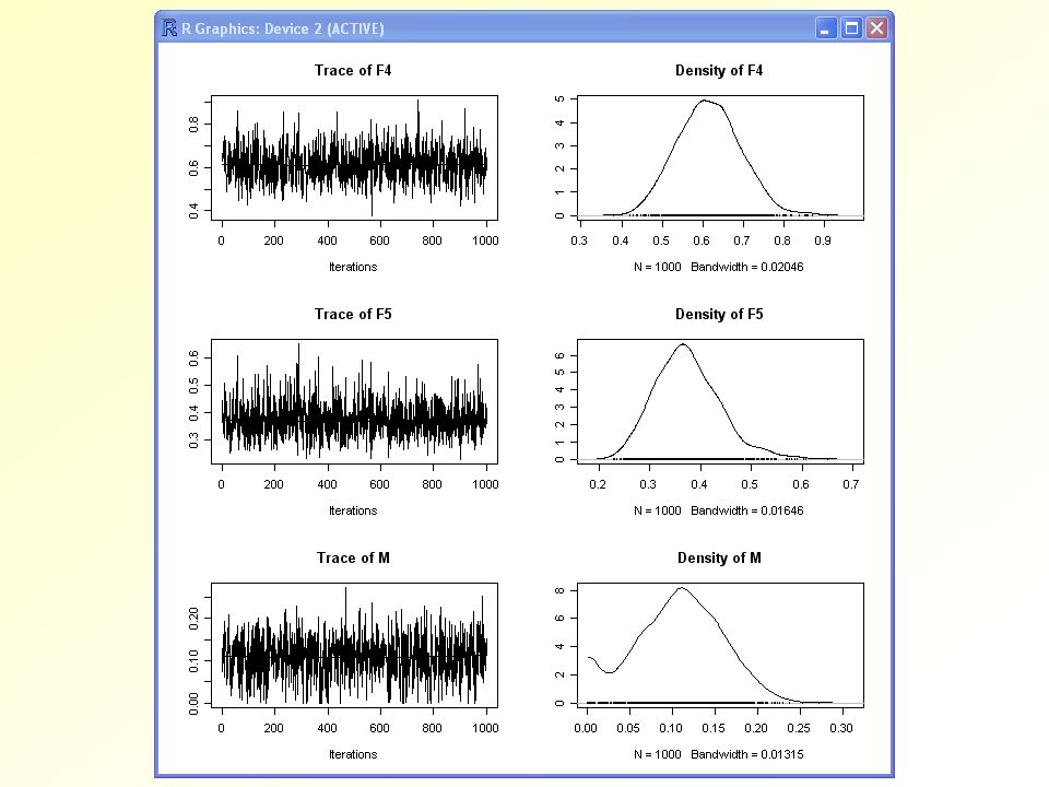
Some basic MCMC diagnostics
Look at trace plot Look at autocorrelation function for chain Calculate “effective sample size” Compare subchain CDFs (if the first and second half differ substantially then chain may be too short Lots of other diagnostics and procedures E.g., parallel chains and formal comparisons

Trace plot example 100,000 steps, sampled every 100

First half Second half Entire chain burn-in excluded
This for lognormal obs error flounder with 100,000 steps, saved every 100, burnin of 100 of saved chain burn-in excluded

Autocorrelation example
This for lognormal obs error flounder with 100,000 chain, save 100 burnin of 100 of saved chain AR(1) shown for comparison (curve)

MCMC Chain Options to make changes to transition rule
-mcgrope p p is the proportion of “fat” tail -mcrb N to 9, smaller = weaker correlation -mcdiag Hessian replaced with Identity -mcmult N Scaler for Hessian -mcnoscale No automatic adj to scaler

Starting and Restarting a Chain
-mcr Restart from where it left off -mcpin fn Start chain at params in fn The output obtained by running with the switches -lprof -prsave (in *.prv) can be useful for this.

Getting MCMC Results into R
To check chains, easiest to simply read the MCMC results into R and to use CODA functions

Steps: 1)Declare your parameters as sdreport_ objects (e.g., sdreport_number parameter1) 2) In procedure section, include the following code if (mceval_phase()) { cout << parameter1 << “ “ << parameter2 << “ “ << endl; } 3) Use "Run ..." command from the ADModel menu. Then in the mini-buffer, you enter the following switches "-mcmc XXX -mcsave YYY" where XXX is the number of MCMC cycles and YYY is how often the cycles are saved. 4) Run the model a second time using the "Run ..." In the minibuffer, you enter the switch "-mceval >> filename" where filename is the name of the file to which you want to save the parameters you are interested in

Open the chain output file in Excel and copy the chain results to the clipboard Use the read.table command in R to copy the data into R Convert to an .mcmc object and use CODA functions

Huge literature on MCMC and Diagnostics
Gelman et al. Bayesian Data Analysis good general source on all things Bayesian Cowles and Carlin, Markov Chain Monte Carlo convergence diagnostics: a comparative review. JASA 91:

Exercises Using models that you have estimated previously (i.e., growth, mortality, recruitment, piecewise) practice using Bayesian methods with both informative and non-informative priors and getting resulting MCMC chains into R and plotting with CODA functions (trace plots, density plots)

Day 3 Questions before proceeding???

Sensitivity to Parameter Starting Values
Why do we care about sensitivity to parameter starting values? Methods for specifying starting values Default values In tpl file In dat file In pin file Precedence between the methods

Why do we care about sensitivity to starting values?
Avoiding local minimums in the likelihood surface If different starting values lead to solution with lower obj. function value, then you were at a local minimum Identifying sensitive parameters If small change to parameter starting value causes large change in results, then you may want to reparameterize model

Default Starting Values
Parameter with unspecified starting value has default starting value of zero Bounded parameter has default starting value which is midway between lower and upper bounds

Specify starting values in tpl file
INITIALIZATION_SECTION log_q -1.0 Must recompile tpl file everytime starting values are changed

Specify starting values in dat file
DATA_SECTION init_number start_log_q PRELIMINARY_CALCS_SECTION log_q = start_log_q; Can change starting values without recompiling tpl file

Specify starting values in pin file
#Example pin file for model with 15 parameters Can change starting values without recompiling tpl file Must specify a starting value for each parameter

Precedence Between Methods
Specifying starting values in dat file takes precedence over pin file and INITIALIZATION_SECTION Specifying starting values in pin file takes precedence over INITIALIZATION_SECTION

Matrix Algebra in ADMB Usual rules of matrix algebra Faster than loops
Also can do element-by-element tasks element-by-element product element-by-element division

Matrix Operations in ADMB
Matrix Addition and Subtraction Element-by-element calculations Commutative: A+B = B+A Associative: A±(B±C)=(A±B)±C Matrix Multiplication and Division Not commutative: A*N usually ≠ N*A ADMB can do both traditional matrix multiplication and element-by-element operations Transpose See Gotelli and Ellison (2004) for a good primer on matrix operations

Matrix Multiplication
Column dimension of A must = Row dimension of N

Array and Matrix Functions
Functions elem_prod and elem_div provide elementwise multiplication and division For vector objects x, y and z z=elem_prod(x,y); //returns zi=xiyi z=elem_div(x,y); //returns zi=xi/yi For matrix objects x, y and z z=elem_prod(x,y); //returns zi,j=xi,jyi,j z=elem_div(x,y); //returns zi,j=xi,j/yi,j

Let’s Try an Example Leslie matrix calculator (following Gotelli 2001)
(very) Simple simulation model Leslie matrix calculator (following Gotelli 2001) No estimation (but dummy parameter still needed in ADMB) Initial abundance-at-age matrix Transition matrix Fecundity Survival

Let’s Try an Example ADMB Tasks: Perform matrix projection
Use a for loop (8 years) Output annual total abundance age-specific abundance Age 1 Age 2 Age 3 Age 4

Advanced Programming Phases Reparameterization to improve estimation

Phases Minimization of objective function can be carried out in phases
Parameter remains fixed at starting value until its phase is reached, then it become active Allows difficult parameters to be estimated when other parameters are “almost” estimated

Phases Specified in PARAMETER_SECTION
init_number x //estimate in phase 1 init_number x(1) //estimate in phase 1 init_number x(-1) //remains fixed init_vector x(1,n,2) //estimate in phase 2 init_matrix x(1,n,1,m,3) //estimate in phase 3

Parameterization Issues
How do you estimate highly correlated parameters? Catchabilities for multiple fisheries Annual recruitments Deviation method Difference method Random walk

Deviation Method Estimate one free parameter
X Estimate m parameters as bounded_dev_vector w1, , wm Then logX1 = logX + w1 logXm = logX + wm

bounded_dev_vector Specified in PARAMETER_SECTION
init_bounded_dev_vector x(1,m,-10,10) Each element must take value between lower and upper bounds -10 < xi < 10 All elements must sum to zero

Difference Method Estimate n free parameters: Then
X1, y1, , yn-1 Then logX1 logX2 = logX1 + y1 logXn = logXn-1 + yn-1

Random Walk Estimate n parameters X1, w1, , wn-1 Then

Time-Varying Von Bertalanffy Growth Model
Asymptotic length varies over time Mean length at age-1 (L1) and Brody growth coefficient (K) are constant over time

Random Walk Model time-varying asymptotic length

Model Parameters Lyr=1…10,age=1 – mean length at age 1 for all years
L,1 – initial asymptotic length K – Brody growth coefficient w1, , w9 – annual deviation of L Lyr=1,age=2…9 – mean length at ages 2…9 for yr. 1

Negative Log Likelihood

Concentrated Negative Log Likelihood

Now to look at the code…..

Overview of Catch-At-Age
CAA estimates of population dynamics CAA predictions of observed data Observed data Negative log likelihood

Basic Relationships in Catch-at-Age Models
Catch in relation to current abundance at fishing and natural mortalities Number at any age in relation to initial cohort strength and cumulative fishing and natural mortality rates Relationship between fishing mortality and fishing effort (catchability)

Observed Data Total annual fishery catch Proportion of catch-at-age
Auxiliary data Fishing effort Survey index of relative abundance Tagging data (to estimate M)

Population Submodel logR+w1 logN1,1+y1 . . . . logN1,n-1+yn-1 logR+w2
Initial numbers at age logR+w2 Recruitment logR+wm

Population Submodel Numbers of fish Survival Total mortality
Fishing mortality Natural mortality

Population Submodel Selectivity Effort Effort error Catchability

Observation Submodel Baranov’s catch equation

Observation Submodel Total catch Observed total catch
Observation error

Observation Submodel Proportion of catch-at-age Numbers sampled at age
Proportions Effective sample size Obs. proportion of catch-at-age

Negative Log Likelihood for Multinomial

Model Parameters R w1, . . . , wm y1, . . . , yn-1 q s1, . . . , sn-1
z1, , zm se Ratio of relative variances (assumed known)

Negative Log Likelihood (ignoring constants)

Now to look at the code…..

Simulating Data

Simulating Data Data simulations are useful for testing models
How well does model perform when processes underlying “reality” are known? The “true” values of parameters and variables can be compared to model estimates Make sure model works before using real world data

Simulating Data “Parameter” values are read in from dat file
“Parameter” values used in estimation model equations to calculate true data Random number generator creates random errors Adding random error to true data gives observed data

Data Generating Model Recruitments generated from white noise process
Input “parameters”

Data Generating Model Numbers at age in first year came from applying mortality to randomly generated recruitments

Input “Parameters” sw M E1, . . . , Em s1, . . . , sn q sz se NE
Must also provide seed for random number generator

Tpl file must still contain:
Data section Parameter section Procedure section objective_function_value One active parameter

Data Generating Model Most of work is done in preliminary calcs section or using local_calcs command Operations involved only need to be run once Use “exit(0);” command at end of local_calcs since no parameters or asymptotic standard errors need to be estimate

Time for some code…..

Simulation Study Simulation study combines a data generating model with a control program to repeatedly fit an estimating model to many simulated data sets This provides replicate model runs to better evaluate an estimating model’s performance Only one replicate normally is available in the real world

Simulation Study Can evaluate how a model performs vs. different underlying “reality” E.g., with different levels of observation error Can evaluate how well different models can fit the same data sets E.g., fit Ricker and Beverton-Holt stock-recruitment models to same data sets Or can use a combination of the two approaches

Simulation Study Practicum
You have seen: Catch-at-age model Data generating model for catch-at-age model Control program for data generating and catch-at-age models Now you need to modify the three programs to run a Monte Carlo simulation study

Simulation Study Practicum
Your simulation study will look at the effects of process error on performance of a catch-at-age model Data sets will be generated using two levels (low and high) of process error for catchability

Let’s code a simulation study…..

Miscellaneous Topics and Tricks
Missing data Advanced ADMB functions Using dat file for flexibility

Missing Data It is not uncommon to have missing years of data in a time series of observed data One solution is to interpolate the missing years of data outside the model fitting process by some ad hoc method E.g., averaging data from the adjacent years A better solution is to allow the model to predict values for the missing data This takes advantage of all the available data

Missing Data Implementation
Use special value to denote missing data in dat file E.g., a value you wouldn’t normally see in real data like -1 Use loops and conditional statements to exclude missing data values from objective function value Otherwise, model will try to match predicted values to the missing data values

Missing Data Multinomial Case
Replace missing data with 0 and it will not contribute to negative log likelihood value

Advanced Functions Filling objects Obtaining shape information
Extracting subobjects Sorting vectors and matrices Cumulative density functions

Filling Objects v.fill(“{1,2,3,6}”); // v=[1,2,3,6]
v.fill_seqadd(1,0.5); // v=[1,1.5,2,2,5] m.rowfill_seqadd(3,1,0.5); // fill row 3 with sequence m.colfill_seqadd(2,1,0.5); // fill column 2 with sequence m.rowfill(3,v); // fill row 3 with vector v m.colfill(2,v); // fill column 2 with vector v

Obtaining Shape Information
i=v.indexmax(); // returns maximum index i=v.indexmin(); // returns minimum index i=m.rowmax(); // returns maximum row index i=m.rowmin(); // returns minimum row index i=m.colmax(); // returns maximum column index i=m.colmin(); // returns minimum column index

Extracting Subobjects
v=column(m,2); // extract column 2 of m v=extract_row(m,3); // extract row 3 of m v=extract_diagonal(m); // extract diagonal elements of m vector u(1,20) vector v(1,19) u(1,19)=v; // assign values of v to elements 1-19 of u --u(2,20)=v; // assign values of v to elements 2-20 of u u(2,20)=++v; // assign values of v to elements 2-20 of u u.shift(5); // new min is 5 new max is 24

Sorting Objects Sorting vectors Sorting matrices
w=sort(v); // sort elements of v in ascending order Sorting matrices x=sort(m,3); // sort columns of m, with column 3 in ascending order

Cumulative Density Functions
For standard normal distribution x=cumd_norm(z); // x=p(Z<=z), Z~N(0,1) Also have CDF for Cauchy distribution cumd_cauchy()

Minnesota AD Model Builder Short Course October 22-24, 2007

Similar presentations

Presentation on theme: "Minnesota AD Model Builder Short Course October 22-24, 2007"— Presentation transcript:

Similar presentations

About project

Feedback

Log in

Auth with social network:

Minnesota AD Model Builder Short Course October 22-24, 2007

Similar presentations

Presentation on theme: "Minnesota AD Model Builder Short Course October 22-24, 2007"— Presentation transcript:

Similar presentations

About project

Feedback