Download presentation
Presentation is loading. Please wait.

1
Geometry and Algebra of Multiple Views
René Vidal Center for Imaging Science BME, Johns Hopkins University Adapted for use in CS by Sastry and Yang Lecture 13. October 11th, 2006 First let us talk about line features. To describe a line in 3-D, we need to specify a base point on the line and a vector indicating the direction of the line. On the image plane we can use a three dimensional vector l to describe the image of a line L. More specifically, if x is the image of a point on this line, its inner product with l is 0.

2
Two View Geometry From two views Why multiple views?
Can recover motion: 8-point algorithm Can recover structure: triangulation Why multiple views? Get more robust estimate of structure: more data No direct improvement for motion: more data & unknowns

3
Why Multiple Views? Cases that cannot be solved with two views
Uncalibrated case: need at least three views Line features: need at least three views Some practical problems with using two views Small baseline: good tracking, poor motion estimates Wide baseline: good motion estimates, poor correspondences With multiple views one can Track at high frame rate: tracking is easier Estimate motion at low frame rate: throw away data

4
Problem Formulation Input: Corresponding images (of “features”) in multiple images. Output: Camera motion, camera calibration, object structure. Here is a picture illustrating the fundamental problem that we are interested in multiple view geometry. The scenario is that we are given multiple pictures or images of some 3D object and after establishing correspondence of certain geometric features such as a point, line or curve, we then try to use such information to recover the relative locations of the camera where these images are taken, as well as recover the 3D structure of the object. measurements unknowns

5
Multiframe SFM as an Optimization Problem
Can we minimize the re-projection error? Number of unknowns = 3n + 6 (m-1) – 1 Number of equations = 2nm Very likely to converge to a local minima Need to have a good initial estimate measurements unknowns
 – 1. Number of equations = 2nm. Very likely to converge to a local minima. Need to have a good initial estimate. measurements. unknowns.")
6
Motivating Examples Image courtesy of Paul Debevec

7
Motivating Examples Image courtesy of Kun Huang

8
Using Geometry to Tackle the Optimization Problem
What are the basic relations among multiple images of a point/line? Geometry and algebra How can I use all the images to reconstruct camera pose and scene structure? Algorithm Examples Synthetic data Vision based landing of unmanned aerial vehicles

9
Projection: Point Features
Homogeneous coordinates of a 3-D point Homogeneous coordinates of its 2-D image Projection of a 3-D point to an image plane Now let me quickly go through the basic mathematical model for a camera system. Here is the notation. We will use a four dimensional vector X for the homogeneous coordinates of a 3-D point p, its image on a pre-specified plane will be described also in homogeneous coordinate as a three dimensional vector x. If everything is normalized, then W and z can be chosen to be 1. We use a 3x4 matrix Pi to denote the transformation from the world frame to the camera frame. R may stand for rotation, T for translation. Then the image x and the world coordinate X of a point is related through the equation, where lambda is a scale associated to the depth of the 3D point relative to the camera center o. But in general the matrix Pi can be any 3x4 matrix, because the camera may add some unknown linear transformation on the image plane. Usually it is denoted by a 3x 3 matrix A(t).
.")
10
Multiple View Matrix for Point Features
WLOG choose frame 1 as reference Rank deficiency of Multiple View Matrix (generic) (degenerate)
 (degenerate)")
11
Geometric Interpretation of Multiple View Matrix
Entries of Mp are normals to epipolar planes Rank constraint says normals must be parallel

12
Multiple View Matrix for Point Features
Mp encodes exactly the 3-D information missing in one image.

13
Rank Conditions vs. Multifocal Tensors
Other relationships among four or more views, e.g. quadrilinear constraints, are algebraically dependent! Two views: epipolar constraint Three views: trilinear constraints

14
Reconstruction Algorithm for Point Features
Given m images of n points The third problem, also the most important one, is how to recover camera configuration from given m images of a set of n points. Using the rank deficiency condition on M, the problem becomes looking for T2, R2, …, Tm, Rm such that the two columns of M are linearly dependent. That is, there exists coefficients alpha^j’s such that the equations hold. I won’t get into the detail how to determine those coefficients alpha^j’s even without knowing all the camera motions. For now, I only tell you their values depend on a choice of coordinate frames. These frames could be either Euclidean, affine or projective. Assuming these coefficients are known, then finding the camera configuration simply becomes a problem of solving a linear equation. This equation have a unique solution if we have in general more than 6 points.

15
Reconstruction Algorithm for Point Features
Given m images of n (>6) points For the jth point SVD Iteration First assume we have m images of n points, where n is at least 8 (actually we need less, but 8 is necessary for initialization using two views linear algorithm). Then for each point, we have a rank condition on the m images for this particular point. If we know all the motions Ri, Ti, then based on its m images, we can find the kernel of the matrix and hence the depth (structure) of the point. On the other hand, for each view, the images of all the points share the same camera motion and hence motion Ri, Ti can be deduced also using SVD if the structure \lambda_I’s are know. If we have perfect data without noise, then first we can pick two views and use these two views to calculate the structure \lambda_I’s for all the points and then calculate the motion for each image. In the presence noise, what do we do? Iteration. Initialized the structure, calculate the motions, then re-calculate the structure and then motions… until it converges. For the ith image SVD
 points. For the jth point. SVD. Iteration. First assume we have m images of n points, where n is at least 8 (actually we need less, but 8 is necessary for initialization using two views linear algorithm). Then for each point, we have a rank condition on the m images for this particular point. If we know all the motions Ri, Ti, then based on its m images, we can find the kernel of the matrix and hence the depth (structure) of the point. On the other hand, for each view, the images of all the points share the same camera motion and hence motion Ri, Ti can be deduced also using SVD if the structure \lambda_I’s are know. If we have perfect data without noise, then first we can pick two views and use these two views to calculate the structure \lambda_I’s for all the points and then calculate the motion for each image. In the presence noise, what do we do Iteration. Initialized the structure, calculate the motions, then re-calculate the structure and then motions… until it converges. For the ith image. SVD.")
16
Reconstruction Algorithm for Point Features
Initialization Set k=0 Compute using the 8-point algorithm Compute and normalize so that Compute as the null space of Compute new as the null space of Normalize so that If stop, else k=k+1 and goto 2.

17
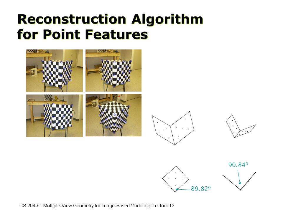
Reconstruction Algorithm for Point Features
90.840 89.820
18
Reconstruction Algorithm for Point Features

19
Multiple View Matrix for Line Features
Homogeneous representation of a 3-D line Homogeneous representation of its 2-D image Projection of a 3-D line to an image plane First let us talk about line features. To describe a line in 3-D, we need to specify a base point on the line and a vector indicating the direction of the line. On the image plane we can use a three dimensional vector l to describe the image of a line L. More specifically, if x is the image of a point on this line, its inner product with l is 0.

20
Multiple View Matrix for Line Features
Point Features Line Features M encodes exactly the 3-D information missing in one image.

21
Multiple View Matrix for Line Features
each is an image of a (different) line in 3-D: Rank =3 any lines Rank =2 intersecting lines Rank =1 same line What is the essential meaning of this rank 2 case? Here is an example explaining it. Consider a family of lines in 3D intersecting at one point p. You then randomly choose the image of any of the lines in the family in each view and form a multiple view matrix. Then this matrix in general has rank 2. We know before that if all the images chosen happen to correspond to the same 3D line, the rank of M is 1. Here, you don’t need to have exact correspondence among those lines, yet you still get some non-trivial constraints among their images… . . . . . . . . .
 line in 3-D: Rank =3. any lines. Rank =2. intersecting lines. Rank =1. same line. What is the essential meaning of this rank 2 case Here is an example explaining it. Consider a family of lines in 3D intersecting at one point p. You then randomly choose the image of any of the lines in the family in each view and form a multiple view matrix. Then this matrix in general has rank 2. We know before that if all the images chosen happen to correspond to the same 3D line, the rank of M is 1. Here, you don’t need to have exact correspondence among those lines, yet you still get some non-trivial constraints among their images…")
22
Multiple View Matrix for Line Features
Continue with constraints that the rank of the matrix M_l imposes on multiple images of a line feature. If rank(M) is 1, it means that all the planes through every camera center and image line intersect at a unique line in 3-D. If the rank is 0, it corresponds to the only degenerate case that all the planes are the same hence the 3-D line is determined only up to a plane on which all the camera centers must lie.
 is 1, it means that all the planes through every camera center and image line intersect at a unique line in 3-D. If the rank is 0, it corresponds to the only degenerate case that all the planes are the same hence the 3-D line is determined only up to a plane on which all the camera centers must lie.")
23
Reconstruction Algorithm for Line Features
Initialization Set k=0 Compute and using linear algorithm Compute and normalize so that Compute as the null space of Compute new as the null space of Normalize so that If stop, else k=k+1 and goto 2.

24
Reconstruction Algorithm for Line Features
Initialization Use linear algorithm from 3 views to obtain initial estimate for and Given motion parameters compute the structure (equation of each line in 3-D) Given structure compute motion Stop if error is small stop, else goto 2.
 Given structure compute motion. Stop if error is small stop, else goto 2.")
25
Universal Rank Constraint
What if I have both point and line features? Traditionally points and lines are treated separately Therefore, joint incidence relations not exploited Can we express joint incidence relations for Points passing through lines? Families of intersecting lines?

26
Universal Rank Constraint
The Universal Rank Condition for images of a point on a line Multi-nonlinear constraints among 3, 4-wise images. Multi-linear constraints among 2, 3-wise images.

27
Universal Rank Constraint: points and lines

28
Universal Rank Constraint: family of intersecting lines
each can randomly take the image of any of the lines: Nonlinear constraints among up to four views . . .

29
Universal Rank Constraint: multiple images of a cube
Three edges intersect at each vertex. . . .

30
Universal Rank Constraint: multiple images of a cube

31
Universal Rank Constraint: multiple images of a cube

32
Universal Rank Constraint: multiple images of a cube

33
Multiple View Matrix for Coplanar Point Features
Homogeneous representation of a 3-D plane Corollary [Coplanar Features] Rank conditions on the new extended remain exactly the same!

34
Multiple View Matrix for Coplanar Point Features
Given that a point and line features lie on a plane in 3-D space: In addition to previous constraints, it simultaneously gives homography:

35
Example: Vision-based Landing of a Helicopter

36
Example: Vision-based Landing of a Helicopter
Landing on the ground Tracking two meter waves

37
Example: Vision-based Landing of a Helicopter

38
General Rank Constraint for Dynamic Scenes
For a fixed camera, assume the point moves with constant acceleration: Here is an example of dynamical scene. We have points in the scene moving with constant velocities or constant accelerations. The 3D location of the point X(t) is just a function of t with coefficients as the initial location X0, initial velocity v0 and constant acceleration a. An equivalent way is to write a fixed 10-dimensional vector \bar{X} containing all the initial location, velocity and acceleration, and a new projection matrix \bar{\Pi} containing the time bases. The image of the point at each time instant t is then characterized by this equation, which is a projection from 10-d space to 2-d image space. Compared with before, we have fixed points in 3d space and the projection is from 3d to 2d. Now the projection is from n-d to 2d. The key point is to decouple time base and constant dynamics and combine the time base in the projection matrix. Now the fixed point in n-d space no longer represent a fixed point 3d space, it represents the trajectory of a point. Then how to characterize the constraints in this new type of projection, actually, as we will see, we can extend this to the most general case where the projection is from n-d space to k-d image space. And now we start to study the algebraic constraints contained in it. Before: Now: Time base
 is just a function of t with coefficients as the initial location X0, initial velocity v0 and constant acceleration a. An equivalent way is to write a fixed 10-dimensional vector \bar{X} containing all the initial location, velocity and acceleration, and a new projection matrix \bar{\Pi} containing the time bases. The image of the point at each time instant t is then characterized by this equation, which is a projection from 10-d space to 2-d image space. Compared with before, we have fixed points in 3d space and the projection is from 3d to 2d. Now the projection is from n-d to 2d. The key point is to decouple time base and constant dynamics and combine the time base in the projection matrix. Now the fixed point in n-d space no longer represent a fixed point 3d space, it represents the trajectory of a point. Then how to characterize the constraints in this new type of projection, actually, as we will see, we can extend this to the most general case where the projection is from n-d space to k-d image space. And now we start to study the algebraic constraints contained in it. Before: Now: Time base.")
39
General Rank Constraint for Dynamic Scenes
Single hyperplane Inclusion Restriction to a hyperplane Intersection Different with the classic 3-d to 2-d space projection in which the features can only be point or line. Now features can be any p-dimensional hyperplane in n-d space. And there are various relationship among multiple features just like point can belong to a line. We call these relationships among features as incidence relations. There are 4 types of incidence relations. First is the most simple case where only one hyperplane is observed in all the images. Second, third, fourth.

40
General Rank Constraint for Dynamic Scenes
Projection from n-dimensional space to k-dimensional space: We define the multiple view matrix as: where ‘s and ‘s are images and coimages of hyperplanes.

41
General Rank Constraint for Dynamic Scenes
Projection from to Single hyperplane Projection from to

42
Summary Incidence relations rank conditions
Rank conditions multiple-view factorization Rank conditions imply all multi-focal constraints Rank conditions for points, lines, planes, and (symmetric) structures.
 structures.")
43
Incidence Relations among Features
“Pre-images” are all incident at the corresponding features Now consider multiple images of a simplest object, say a cube. All the constraints are incidence relations, are all of the same nature. Is there any way that we can express all the constraints in a unified way? Yes, there is. . . .

44
Traditional Multifocal or Multilinear Constraints
Given m corresponding images of n points This set of equations is equivalent to Multilinear constraints among 2, 3, 4 views

45
Multiview Formulation: The Multiple View Matrix
Point Features Line Features

Similar presentations


Correspondence geometry: Given an image point x in the first view, how does this constrain the position of the corresponding point.>")
: Given 2D point matches in two or more images, where are the corresponding.>")


