Download presentation
Presentation is loading. Please wait.

1
Multi-view geometry

2
Multi-view geometry problems
Structure: Given projections of the same 3D point in two or more images, compute the 3D coordinates of that point ? Structure from motion solves the following problem: Given a set of images of a static scene with 2D points in correspondence, shown here as color-coded points, find… a set of 3D points P and a rotation R and position t of the cameras that explain the observed correspondences. In other words, when we project a point into any of the cameras, the reprojection error between the projected and observed 2D points is low. This problem can be formulated as an optimization problem where we want to find the rotations R, positions t, and 3D point locations P that minimize sum of squared reprojection errors f. This is a non-linear least squares problem and can be solved with algorithms such as Levenberg-Marquart. However, because the problem is non-linear, it can be susceptible to local minima. Therefore, it’s important to initialize the parameters of the system carefully. In addition, we need to be able to deal with erroneous correspondences. Camera 1 Camera 3 Camera 2 R1,t1 R3,t3 R2,t2 Slide credit: Noah Snavely

3
Multi-view geometry problems
Stereo correspondence: Given a point in one of the images, where could its corresponding points be in the other images? Structure from motion solves the following problem: Given a set of images of a static scene with 2D points in correspondence, shown here as color-coded points, find… a set of 3D points P and a rotation R and position t of the cameras that explain the observed correspondences. In other words, when we project a point into any of the cameras, the reprojection error between the projected and observed 2D points is low. This problem can be formulated as an optimization problem where we want to find the rotations R, positions t, and 3D point locations P that minimize sum of squared reprojection errors f. This is a non-linear least squares problem and can be solved with algorithms such as Levenberg-Marquart. However, because the problem is non-linear, it can be susceptible to local minima. Therefore, it’s important to initialize the parameters of the system carefully. In addition, we need to be able to deal with erroneous correspondences. Camera 1 Camera 3 Camera 2 R1,t1 R3,t3 R2,t2 Slide credit: Noah Snavely

4
Multi-view geometry problems
Motion: Given a set of corresponding points in two or more images, compute the camera parameters Structure from motion solves the following problem: Given a set of images of a static scene with 2D points in correspondence, shown here as color-coded points, find… a set of 3D points P and a rotation R and position t of the cameras that explain the observed correspondences. In other words, when we project a point into any of the cameras, the reprojection error between the projected and observed 2D points is low. This problem can be formulated as an optimization problem where we want to find the rotations R, positions t, and 3D point locations P that minimize sum of squared reprojection errors f. This is a non-linear least squares problem and can be solved with algorithms such as Levenberg-Marquart. However, because the problem is non-linear, it can be susceptible to local minima. Therefore, it’s important to initialize the parameters of the system carefully. In addition, we need to be able to deal with erroneous correspondences. ? Camera 1 ? Camera 3 Camera 2 ? R1,t1 R3,t3 R2,t2 Slide credit: Noah Snavely

5
Two-view geometry

6
Epipolar geometry Baseline – line connecting the two camera centers
X x x’ Baseline – line connecting the two camera centers Epipolar Plane – plane containing baseline (1D family) Epipoles = intersections of baseline with image planes = projections of the other camera center = vanishing points of the motion direction
 Epipoles. = intersections of baseline with image planes. = projections of the other camera center. = vanishing points of the motion direction.")
7
The Epipole Photo by Frank Dellaert

8
Epipolar geometry Baseline – line connecting the two camera centers
X x x’ Baseline – line connecting the two camera centers Epipolar Plane – plane containing baseline (1D family) Epipoles = intersections of baseline with image planes = projections of the other camera center = vanishing points of the motion direction Epipolar Lines - intersections of epipolar plane with image planes (always come in corresponding pairs)
 Epipoles. = intersections of baseline with image planes. = projections of the other camera center. = vanishing points of the motion direction. Epipolar Lines - intersections of epipolar plane with image planes (always come in corresponding pairs)")
9
Example: Converging cameras

10
Example: Motion parallel to image plane

11
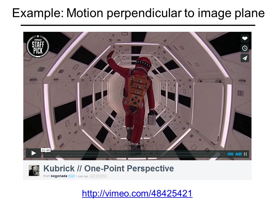
Example: Motion perpendicular to image plane

12
Example: Motion perpendicular to image plane
Points move along lines radiating from the epipole: “focus of expansion” Epipole is the principal point

13
Example: Motion perpendicular to image plane
14
Epipolar constraint X x x’ If we observe a point x in one image, where can the corresponding point x’ be in the other image?

15
Epipolar constraint X X X x x’ x’ x’ Potential matches for x have to lie on the corresponding epipolar line l’. Potential matches for x’ have to lie on the corresponding epipolar line l.

16
Epipolar constraint example

17
Epipolar constraint: Calibrated case
X x x’ Intrinsic and extrinsic parameters of the cameras are known, world coordinate system is set to that of the first camera Then the projection matrices are given by K[I | 0] and K’[R | t] We can multiply the projection matrices (and the image points) by the inverse of the calibration matrices to get normalized image coordinates:
 by the inverse of the calibration matrices to get normalized image coordinates:")
18
Epipolar constraint: Calibrated case
X = (x,1)T x x’ = Rx+t t R X’ is X in the second camera’s coordinate system We can identify the non-homogeneous 3D vectors X and X’ with the homogeneous coordinate vectors x and x’ of the projections of the two points into the two respective images The vectors Rx, t, and x’ are coplanar
T. x. x’ = Rx+t. t. R. X’ is X in the second camera’s coordinate system. We can identify the non-homogeneous 3D vectors X and X’ with the homogeneous coordinate vectors x and x’ of the projections of the two points into the two respective images. The vectors Rx, t, and x’ are coplanar.")
19
Epipolar constraint: Calibrated case
X x x’ = Rx+t Essential Matrix (Longuet-Higgins, 1981) The vectors Rx, t, and x’ are coplanar
 The vectors Rx, t, and x’ are coplanar.")
20
Epipolar constraint: Calibrated case
X x x’ E x is the epipolar line associated with x (l' = E x) ETx' is the epipolar line associated with x' (l = ETx') E e = 0 and ETe' = 0 E is singular (rank two) E has five degrees of freedom
 ETx is the epipolar line associated with x (l = ETx ) E e = 0 and ETe = 0. E is singular (rank two) E has five degrees of freedom.")
21
Epipolar constraint: Uncalibrated case
X x x’ The calibration matrices K and K’ of the two cameras are unknown We can write the epipolar constraint in terms of unknown normalized coordinates:

22
Epipolar constraint: Uncalibrated case
X x x’ Fundamental Matrix (Faugeras and Luong, 1992)
")
23
Epipolar constraint: Uncalibrated case
X x x’ F x is the epipolar line associated with x (l' = F x) FTx' is the epipolar line associated with x' (l' = FTx') F e = 0 and FTe' = 0 F is singular (rank two) F has seven degrees of freedom
 FTx is the epipolar line associated with x (l = FTx ) F e = 0 and FTe = 0. F is singular (rank two) F has seven degrees of freedom.")
24
The eight-point algorithm
Minimize: under the constraint ||F||2=1

25
The eight-point algorithm
Meaning of error sum of squared algebraic distances between points x’i and epipolar lines F xi (or points xi and epipolar lines FTx’i) Nonlinear approach: minimize sum of squared geometric distances
 Nonlinear approach: minimize sum of squared geometric distances.")
26
Problem with eight-point algorithm

27
Problem with eight-point algorithm
Poor numerical conditioning Can be fixed by rescaling the data

28
The normalized eight-point algorithm
(Hartley, 1995) Center the image data at the origin, and scale it so the mean squared distance between the origin and the data points is 2 pixels Use the eight-point algorithm to compute F from the normalized points Enforce the rank-2 constraint (for example, take SVD of F and throw out the smallest singular value) Transform fundamental matrix back to original units: if T and T’ are the normalizing transformations in the two images, than the fundamental matrix in original coordinates is T’T F T
 Center the image data at the origin, and scale it so the mean squared distance between the origin and the data points is 2 pixels. Use the eight-point algorithm to compute F from the normalized points. Enforce the rank-2 constraint (for example, take SVD of F and throw out the smallest singular value) Transform fundamental matrix back to original units: if T and T’ are the normalizing transformations in the two images, than the fundamental matrix in original coordinates is T’T F T.")
29
Comparison of estimation algorithms
8-point Normalized 8-point Nonlinear least squares Av. Dist. 1 2.33 pixels 0.92 pixel 0.86 pixel Av. Dist. 2 2.18 pixels 0.85 pixel 0.80 pixel

30
From epipolar geometry to camera calibration
Estimating the fundamental matrix is known as “weak calibration” If we know the calibration matrices of the two cameras, we can estimate the essential matrix: E = K’TFK The essential matrix gives us the relative rotation and translation between the cameras, or their extrinsic parameters

Similar presentations


Correspondence geometry: Given an image point x in the first view, how does this constrain the position of the corresponding point.>")
: Given 2D point matches in two or more images, where are the corresponding.>")


