2. Dynamic Link Matching Hamid Reza Vaezi Mohammad Hossein Rohban Neural Networks Spring 2007

3. Outline Introduction –Topography based Object Recognition Basic Dynamic Link Matching –Ideas –Formalization Improved Dynamic Link Matching –Principles –Differential Equations Implementation Experiments and Results

4. Introduction Visual Image in Conventional Neural Net –Image is represented by Vectors –Ignoring spacial relation Solution: preprocess, Neocognitron. Which pattern?

5. Labeled Graph Data Structure to overcome aforementioned problem Object Representation First used in Neural Net by Dynamic Link Matching Structure: –Set of Nodes: containing local features. –Set of Edged: connecting nodes.

6. Labeled Graph Feature Space: set of all local features. –Image: Absolute information extracted from small patch of image such as: Color, Texture, Dimension of edge. –Acoustic signal: onset, offset or energy in particular frequency channel. Sensory Space: space from which relational features are extracted –Image: Frequency axes or spatial relations. –Acoustic signal: frequency or time.

7. Sample Labeled Graph Dashed Line: proximity in Sensory Space. Solid Line: Proximity in feature Space.

8. Labeled Graph Matching Object Recognition Detecting Symmetry Finding partial identity

9. Object Recognition Object Recognition Problem –Given a test image of an object and a gallery of object images, find the matching images in the gallery. Topography based solutions –Use ordering and local intensity of images –Find a 1 – 1 mapping between regions of two images.

10. DLM Principles Dynamic Link Matching –Konen & Von Der Malsburg (1992 – 1993) –Konen & Vorbrüggen (1993) It contain 4 principle: Correlation Encodes Neighborhood –Two neighbor nodes have correlated output in both layers. Layer Dynamics Synchronize –Two blobs should align and synchronize in two layers if model and image represent the same object in last iterations. Synchrony is Robust against noise Synchrony Structures Connectivity –Use weight plasticity to improve region mapping.

11. DLM Idea –Consider two layered neural network First layer represents input image (Image Layer) Second layer represents gallery images (Model Layer) –Weight from i th neuron in first layer to j th neuron in second layer, represents degree of matching between corresponding i th region and j th region. –Each neuron stores a local wavelet response in the corresponding pixel of the image –Output of each neuron represents image scanning.

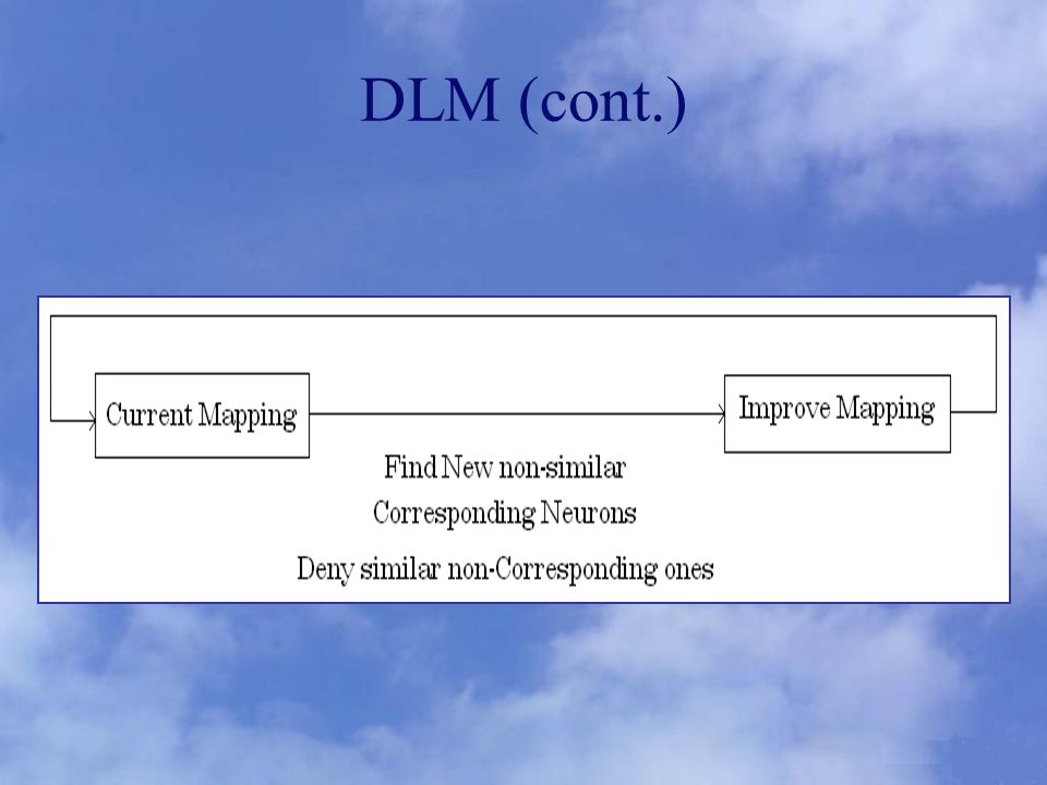
12. DLM (cont.)

13. Idea (cont.) –Create a blob in 1 st layer (Image Layer) a set of neighbor regions with high output –1 st layer sends its output to 2 nd layer (Model Layer) Sigmoid on sum of weighted inputs model. –Neighbor neurons in 2 nd layer with high activities (if exist), amplify their activities. (topography!) –If two nodes in two layers fire simultaneously, strengthen their connection. –Repeat the above process –After a while if there is high blob activity in 2 nd layer, it is concluded that two images represent the same object.

14. DLM (cont.)

16. Notations –h 0 i = i th neuron of 1 st layer –h 1 j = j th neuron of 2 nd layer –I i (t) iid random noise, J i = jet connected to i th node –  (.) sigmoid activation function, S  = similarity Measure –W ij weight of connection between j th to i th neuron

17. DLM (cont.) Local Excitation Lack of excitation leads to decay in h(t)

18. DLM (cont.) If two nodes in two layers are correlated, increase their connection strength Weights converging on a 2 nd layer neuron are normalized. Having changed connections, run differential equations again. Repeat until some predefined number of iterations. If activity on 2 nd layer is high, two images are considered equivalent.

19. Drawbacks Need accurate schedule for layer dynamics, rather than being autonomous. Information about correspondence of blobs would be lost in next iteration, after altering weights. Slow process, many iterations, each with solving two differential equations iteratively. In practice can not handle a gallery with more than 3 images.

20. Solution L. Wiskott (1995) changed this architecture. Ideas : –Two differential equations are considered. –Each model a blob in a layer. –Equations are solved only once. –Blobs are moving almost continuously, thus preserving information from previous iteration. –Attention blob concept is introduced Do not scan all points in the main image, but regions with high activity. –Connections are bidirectional for blob alignment and attention blob formation. –Much faster and accurate, on 20, 50, 111 model galleries.

21. Blob Formation Local Excitation Global Inhibition i = (0,0), (0, 1), (0, 2), …

22. Blob Formation (cont.) Formation equation can be written as :

23. Blob Formation (cont.) Blob can arise only if  h <1. Lower  h leads to larger blobs. Using this form of activation function : –Vanishes for negative value, so no oscillation. –Higher slope for smaller values ease blob formation from small noise values.

24. Blob Formation (cont.) Creating blob in this way makes neighbor neurons be highly correlated in temporal domain. (1 st Principle) –Neighbor neurons excites almost in the same way In order to test 2 nd principle (Synchronization) we need moving blobs. We may store paths of the blobs and move away.

25. Blob Mobilization We may change equations : s i (t) acts as a memory and is called self inhibitory.  is a varying decay constant. Rewriting the formula of s :

26. Blob Mobilization (cont.)  takes two values and so has two functions : –When h>s, it is a high positive value. –When h<s, it is a low positive value. Functions : –When h>s, blob has recently been arrived, increasing s, makes blob move away. –When h<s, blob has recently been moved away, softly decreasing s, cause blob not to move to its recent place.

27. Blob Mobilization (cont.) Why the blob sometimes jumps?

28. Layer Interaction Neurons of two layers are also excited according to activity of the “known corresponding neurons” in the other layer : W ij pq codes synchrony (mapping) of node j in layer q to node i in layer p.

29. Layer Interaction (cont.) Left : Early non-synchronized case Right : Final synchronized –There is a blob in the location of maximal input, in output layer.

30. Link Dynamics Computing neurons activity using “know mapping matrix”, we want to approximate a new mapping matrix. S  measures similarity, J is the jet connected to each neuron,  is a heavy-side function

31. Link Dynamics (cont.) The synaptic weights grow exponentially controlled by the correlation between neuron activities. If one link in connections converging on node i (in output layer) grows beyond its initial value, all these connections will be reduced. Best link will be preserved in this case.

32. Attention Dynamics Image layer is usually larger than model layer. Need to restrict moving area of blob.

33. Attention Dynamics (cont.) Neurons with corresponding activity value beyond  ac will be strengthen. Activity value of attention blob should change slowly. Attention blob get excited by corresponding running blob : moving toward active regions.

34. Attention Dynamics (cont.)

36. Recognition Dynamics The most similar model cooperates most successfully and is the most active one.

37. Parameters

38. Bidirectional Connections With unidirectional connections, one blob would run behind the other. Connection –Model  Image : Moving attention blob appropriately. –Image  Model : Discrimination cue as to which model best fits the image.

39. Max vs. Summation Why did we use max j instead of summing on j variable? –Many connections converging on a neuron, only one is a correct connection. Using sum decreases neuron SNR. –Dynamic range of inputs do not change much, after re- organization of weights.

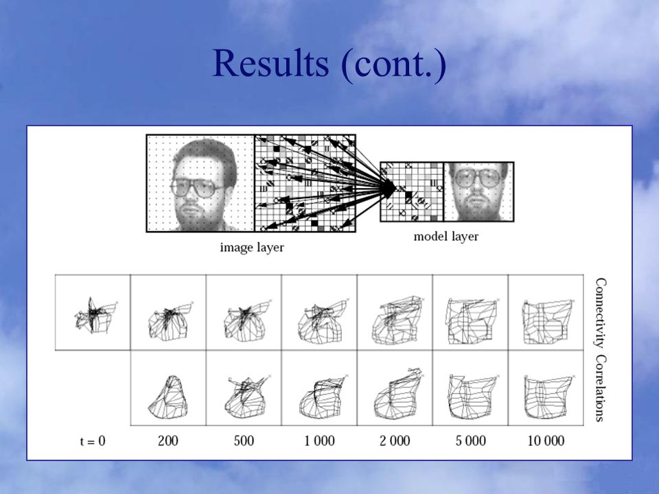
40. Experiments Gallery database of 111 persons. –One neutral image of frontal view. –One frontal view with different facial expression. –Two rotated in depth image with 15 and 30 degrees of rotation. –Neutral image acts as model images. –Other images acts as test images. Model is 10  10 and image is 16  17. Grids are moved to have nodes in areas such as eyes, mouth and nose.

41. Experiments (cont.) DLM is somehow changed : –For 1000 first time steps, no weight correction is done, to stabilize attention blob. It take 10-15 min to recognize faces on a Sun SPARC station, with a 50 MHz processor. Seems much far from acting real time.

42. Results

43. Results (cont.)

46. Drawbacks Path of running blob is not random, but is dependent on initial random state of neurons and activity of the other layer. Thus certain paths may dominate and topology is encoded inhomogenously : strongly along typical paths and weakly elsewhere. Solution : –Other ways of encoding topology : plane waves. –Cause slow running of the process.

47. Conclusions DLM works based on topology coding. Topology is coded by blobs. Two layer architecture tries to find the mapping between two topologies. Topologies are mapped using correlation of neurons. Models with highest activity are chosen. Proposed method needs no training data to perform intelligently.

48. References L. Wiskott, “Labeled Graphs and Dynamic Link Matching for Face Recognition and Scene Analysis,” PhD Thesis, Ruhr University, Bochum, 1995. W. Konen, C. Von Der Malsburg, “Learning to Generalize from Single Examples in the Dynamic Link Architecture”, Neural Computation, 1993.

49. Thanks for your attention! Any Question ?