1. Significance Tests in practice Chapter 12

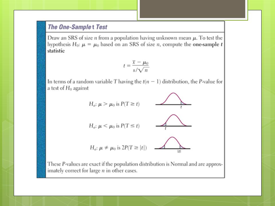
2. 12.1 Tests about a population mean  When we don’t know the population standard deviation σ, we perform a one sample T test instead of a Z test  We get a “T calc” (instead of a Z calc) and the formula is the same except we put in the standard deviation S x of our sample as a replacement for σ

3. Interpretation and P values  same as Z interval, except if you are using the tables, look up “T star” to find the critical T value you need to beat. I recommend the calculator though…  The P value is from your calculated T to the tail. If it is a 2 tailed test, remember this gets doubled!

5. T test on calc  Go to Stat/Tests choose 2: T-test. Enter either data or Stats (just like Z test)

6. Example: Diversity (P. 750)  An investor with a stock portfolio sued his broker b/c lack of diversification in his portfolio led to poor performance. The table gives the rates of return for the 39 months that the account was managed by the broker. Consider the 39 monthly returns as a random sample from the monthly returns the broker would generate if he managed the account forever. Are these returns compatible with a population of μ=.95%, The S&P 500 average?

7. -8.361.63-2.27-2.93-2.70-2.93-9.14-2.646.82-2.35-3.586.137 - 15.2 5 -8.66-1.03-9.16-1.25-1.22- 10.2 7 -5.11-.80-1.441.28-.654.34 12.2 2 -7.21-.097.345.04-7.24-2.14-1.01-1.4112.0 3 -2.564.332.35 Step 1 : Hypothesis- (Where μ is the mean return for all possible months that the broker could manage this account) H 0 : μ =.95 H A : μ ≠.95 Step 2 : Conditions- Since we do not know σwe must use a one- sample t test. Now we check conditions: SRS- We are told this in problem Normality: Sample is large enough (39) so CLT applies Independence: We must treat the 39 monthly returns as independent observations from the population of months in which the broker could have managed the account.

8.  Step 3: Calculations-  Test Statistic: (-1.10 -.95) / (5.99/√39) = -2.14  P value: df are 39-1 = 38. Since we are performing a 2-tailed test, our P-value is.039 (can be done on calc, or on table- if doing table, make sure to double the area under the curve b/c of 2 tailed!)  Step 4: Interpretation: The mean monthly return on investment for this client’s account was -1.1% for this period (this is our x bar). This is significantly difference at the alpha =.05 level of the S&P 500 for the same period (t = - 2.14, P<.05)

9. Paired T Test – Testing the differences Example: Sweet Cola (P. 746)  Diet colas use artificial sweeteners which gradually lose their sweetness overtime. Trained tasters sip cola and give it a “sweetness scale rating” of 1 to 10. Then it is stored for 4 months and tested again. The differences in sweetness score are listed (The bigger the differences, the bigger the loss of sweetness, negative value means it gained sweetness) 2.4.72-.42.2-1.31.21.12.3

10.  Step 1 : Hypothesis- since we care about the difference, μ before -μ after = μ diff  H 0 : μ diff = 0 “The mean sweetness loss for the population of tasters is zero”  H A : μ diff > 0 “The mean sweetness loss for the population of tasters is positive. The cola seems to be losing sweetness in storage  Step 2 : Conditions- Since we do not know the standard deviation of sweetness loss in the population of tasters, we must use a one- sample t test. Now we check conditions:  SRS- assume the 10 tasters are randomly selected  Normality: 10 is too small a sample so we check our normal probability plot

11.  It is slightly left skewed, but no gaps/outliers so we proceed with caution  Independence: we assume there are more then 10x10 = 100 tasters in the population

12.  Step 3: Calculations  Test Statistic- The basic statistics are  X bar diff = 1.01 and S diff = 1.196  T calc = (1.02 – 0)/ (1.196/√10) = 2.70  P value: degrees of freedom are 10-1 = 9 for alpha =.05, p =.0123

13.  Step 4: Interpretation- A P-value this low gives strong evidence against the null hypothesis. We reject H 0 and conclude that the cola has lost sweetness during storage  *Remember the 3C’s! (Conclusion, connection, context)

14. Robustness and Power  Recall that t procedures are robust against non-normality of the population except when outliers or strong skewness are present (skewness is more serious). As the sample size increases, the CLT ensures that our distribution of sample means approximates normality.  Again, calculating power is not in this course, but remember we can still commit the same type I / type II errors when rejecting (or failing to reject) the null.

15. 12.2 Tests about a population proportion  Remember, when the 3 conditions are met (SRS, Normality, and Indep.), the sampling distribution of p hat is approximately Normal with mean equal to rho and standard deviation = √(pq/n)

16. Note: In the standard error (denominator of test statistic) we use the values of our assumed null hypothesis- this is different from the standard error of the CI where we used sample proportion values!

17. One proportion z on calc  Stat- Test – 1-propZtest put in:  Rho  x = the count (number of successes in your sample)  n = number of people in your sample  choose one-tailed or 2 tailed hypothesis  calculate

18. Example (P. 767) work stress  Job stress poses a major threat to the health of workers. A national survey or restaurant employees found that 75% said that work stress had a negative impact on their personal lives. A random sample of 100 employees from a large restaurant chain finds that 68 answer “yes” when asked “Does work stress have a negative impact on your personal life?”. Is this good reason to think that the proportion of all employees in this chain who would say “yes” differs from the national proportion of ρ=.75?

19.  Hypothesis: we want to test a claim about ρ, the true proportion of this chain’s employees who would say that work stress has a negative impact on their personal lives.  H 0 : ρ=.75 H A : ρ ≠.75  Conditions: We should use a one-proportion Z test if the conditions are met  SRS: we are told in problem  Normality: The expected number of “yes” and “no” responses are (100)(.75) = 75 and (100)(.25) = 25 respectively. Both are at least 10 s  Independence: We assume the chain has at least 10(100) = 1000 employees

20.  Calculations  Test Statistic:  P value =.1052 (if you do normalcdf, remember to double your value b/c this is a 2 tailed test! so 2x.0526!) BUT! MUCH easier to do on Calc though and not use NormalCDF! Try it  Interpretation There is over a 10% chance of obtaining a sample result as unusual as or even more unusual than we did (p hat =.68) when the null is true so we have insufficient evidence to suggest that the proportion of this chain restaurant’s employees who suffer from work stress is different from the national survey result,.75

21. Confidence Intervals  using the info from that same example, if we were to calculate a 95% CI (.59,.77)  by hand, using formula:  Note: the CI standard error uses the sample proportions, but in the test statistic formula we use the value assumed in the null hypothesis  Using calc is easier though: choose 1 prop z int  Interpretation: We are 95% confident that between 59% and 77% of the restaurant chain’s employees feel that work stress is damaging their personal lives.