1. Mean = 41.21Median = 42.5s = 7.59 x - 1s – x + 1s – Assignment #1

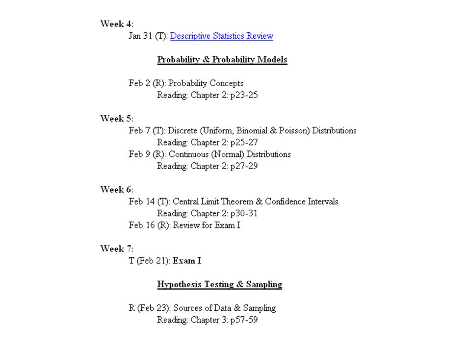
2. Course Schedule

4. Probabilities in Geography The analyses of many problems (daily or geographic) are often based on probabilities, such as: What are the “chances” of having rain over the weekend? What is the “likelihood” that the 100-year flood will occur within the next ten years? How “likely” is it that a pixel on a satellite image is correctly classified or misclassified?

5. Probability & Probability Distribution We summarize a sample statistically and want to make some inferences about the population (e.g., what proportion of the population has values within a given range) The concept of probability is the key to making statistical inferences by sampling a population What we are doing is trying to ascertain the probability of an event having a given outcome This requires us to be able to specify the distribution of a variable before we can make inferences

6. Probability & Probability Distributions Previously, we looked at some proportions of area under the normal curve: Source: Earickson, RJ, and Harlin, JM. 1994. Geographic Measurement and Quantitative Analysis. USA: Macmillan College Publishing Co., p. 100.

7. Probability & Probability Distributions BUT before we could use the normal curve, we have to find out if this is the right distribution for our variable … While many natural phenomena are normally distributed, there are other phenomena that are best described using other distributions Background on probabilities (terminology & rules), and a few useful distributions: Discrete distributions: Binomial and Poisson Continuous distributions: Normal and its relatives

8. Probability-Related Concepts An event – Any phenomenon you can observe that can have more than one outcome (e.g., flipping a coin) An outcome – Any unique condition that can be the result of an event (e.g., flipping a coin: heads or tails), a.k.a simple event or sample points Sample space – The set of all possible outcomes associated with an event –e.g., flip a coin – heads (H) and tails (T) –e.g., flip a coin twice – HH, HT, TH, TT

9. Associated with each possible outcome in a sample space is a probability Probability is a measure of the likelihood of each possible outcome Probability measures the degree of uncertainty Each of the probabilities is greater than or equal to zero, and less than or equal to one The sum of probabilities over the sample space is equal to one Probability-Related Concepts

10. Probability – Examples Example I – Flip a coin –Two possible outcomes: “heads”, “tails” –Each outcome is equally likely –“heads” and “tails” have the same probability (0.5) –The sum of probabilities over the sample space is one –# of “heads” and # of “tails” will be nearly equal

11. Probability – Examples Example II – Flip a coin twice –Four outcomes are equally likely –Tosses of the coin are independent –Each outcome has probability 1/4 –The probability of a head on Flip 1 and a head on Flip 2 is 1/2 * 1/2 = 1/4 OutcomeFirst flipSecond flip 1Heads 2 Tails 3 Heads 4Tails

12. How To Assign Probabilities to Experimental Outcomes? There are numerous ways to assign probabilities to the elements of sample spaces Classical method assigns probabilities based on the assumption of equally likely outcomes Relative frequency method assigns probabilities based on experimentation or historical data Subjective method assigns probabilities based on the assignor’s judgment or belief

13. Classical Method This approach assumes that each outcome is equally likely If an experiment has n possible outcomes, this method would assign a probability of 1/n to each outcome. It is an appropriate way to assign probabilities to the outcomes in special kinds of experiments

14. Classical Method Example I: Rolling a die Sample Space: S = {1, 2, 3, 4, 5, 6} Probabilities: Each sample point has a 1/6 chance of occurring.

15. Classical Method Example II – Flip four coins –Let “0” represent “heads” and “1” represents “tails” –For each toss, the probability of “heads” or “tails” is ½ –Assuming that outcomes of the four tosses are independent from one another –Sixteen possible outcomes × × ½ ½ ½ ½ Probability of each outcome: ½ * ½ * ½ * ½ = 1/16 = 0.0625 0000010010001100 0001010110011101 0010011010101110 0011011110111111

16. Relative Frequency Method The second way is to assign them on the basis of relative frequencies Example –Given a weather pattern, a meteorologist may note that in 65 out of the last 100 times that such a pattern prevailed there was measurable precipitation the next day –If there were such a weather pattern today, what would the probability of having rain tomorrow be? –The possible outcomes – rain or no rain tomorrow – are assigned probabilities of 0.65 and 0.35, respectively

17. Subjective Method When extreme weather conditions occur it might be inappropriate to assign probabilities based solely on historical data We can use any data available as well as our experience and intuition, but ultimately a probability value should express our degree of belief that the experimental outcome will occur The best probability estimates often are obtained by combining the estimates from the classical or relative frequency approach with the subjective estimates.

18. Probability Rules Rules for combining multiple probabilities A useful aid is the Venn diagram - depicts multiple probabilities and their relations using a graphical depiction of sets The rectangle that forms the area of the Venn Diagram represents the sample (or probability) space, which we have defined above Figures that appear within the sample space are sets that represent events in the probability context, & their area is proportional to their probability (full sample space = 1) AB

19. Probability Rules We can use a Venn diagram to describe the relationships between two sets or events, and the corresponding probabilities The union of sets A and B (written symbolically is A  B) is represented by the areas enclosed by set A and B together, and can be expressed by OR (i.e. the union of the two sets includes any location in A or B) The intersection of sets A and B (written symbolically as A  B) is the area that is overlapped by both the A and B sets, and can be expressed by AND (i.e. the intersection of the two sets includes locations in A AND B) AB AB  

20. Addition Rule If sets A and B do not overlap in the Venn diagram, the sets are disjoint, and this represents a case of two independent, mutually exclusive events The union of sets A and B here uses the addition rule, where P(A  = P(A) + P(B) You can think of this in terms of areas of the events, where the union in this case is simply the sum of the areas The intersection of sets A and B here results in the empty set (symbolized by  ), because at no point do the circles overlap AB AB P(A  = P(A) + P(B) P(A  = 

21. Probability Rules The union of sets A and B here uses the addition rule, where P(A  = P(A) + P(B) P(A  = 2/6 + 2/6 P(A  = 4/6 = 2/3 = 0.67 The outcomes represented here are mutually exclusive, thus there is no intersection between sets A and B, thus P(A  =  AB AB P(A  = P(A) + P(B) P(A  =  For example, suppose set A represents a roll of 1 or 2 on a 6-sided die, so P(A)=2/6, and set B represents a roll of 3 or 4, so P(B)=2/6

22. Probability Rules – General Addition Rule If sets A and B do overlap in the Venn diagram, the sets are independent but not mutually exclusive The union of sets A and B here is P(A  = P(A) + P(B) - P(A  because we do not wish to count the intersection area twice, thus we need to subtract it from the sum of the areas of A and B when taking the union of a pair of overlapping sets The intersection of sets A and B here is calculated by taking the product of the two probabilities, a.k.a. the multiplication rule: AB AB P(A  = P(A) * P(B)  P(A  = P(A) + P(B) - P(A  

23. General Addition Rule Consider set A to give the chance of precipitation at P(A)=0.4 and set B to give the chance of below freezing temperatures at P(B)=0.7 The intersection of sets A and B here is P(A  = P(A) * P(B) P(A  = 0.4 * 0.7 = 0.28 This expresses the chance of snow at P(A  = 0.28 The union of sets A and B here is P(A  = P(A) + P(B) - P(A  P(A  = 0.4 + 0.7 – 0.28 = 0.82 This expresses the chance of below freezing temperatures or precipitation occurring at P(A  = 0.82 AB P(A  = P(A) + P(B) - P(A   AB P(A  = P(A) * P(B) 

24. Complement Consider set A to give the chance of precipitation at P(A)=0.4 and set B to give the chance of below freezing temperatures at P(B)=0.7 The complement of set A is P(A’  = 1 - P(A) P(A’  = 1 – 0.4 = 0.6 This expresses the chance of it not raining or snowing at P(A’  = 0.6 The complement of the union of sets A and B is P(A  ’ = 1 – [P(A) + P(B) - P(A  P(A  ’ = 1 – [0.4 + 0.7 – 0.28] = 0.18 This expresses chance of it neither raining nor being below freezing at P(A  ’ = 0.18 P(A’  = 1 - P(A) P(A  ’ = 1 – [P(A) + P(B) - P(A  AA’ AB P(A  ’

25. Probability Rules We can also encounter the situation where set A is fully contained within set B, which is equivalent to saying that set A is a subset of set B: For example, set A might represent precipitation events with >= 5 inches, whereas set B denotes any events with >= 1 inch  A is contained with B because anytime A occurs, B occurs as well In probability terms, this situation occurs when outcome B is a necessary precondition for outcome A to occur, although not vice-versa (in which case set B would be contained in set A instead) A B

26. Probability – Example Example – # of malls within cities City # of Malls A1 B4 C4 D4 E2 F3 We might wonder if we randomly pick one of these six cities, what is the probability (chance) that it will have n malls? Sample Space Each count of the # of malls in a city is an event

27. Random Variables What we have here is a random variable – defined as a function that associates a unique numerical value with every outcome of an experiment To put this another way, a random variable is a function defined on the sample space  this means that we are interested in all the possible outcomes A random variable X is a rule that assigns a numerical value to each outcome in the sample space of an experiment

28. Random Variables The value of the random variable will vary from trial to trial as the experiment is repeated We use an uppercase letter to denote a random variable and a lowercase letter to denote a particular value of the variable A random variable can be classified as being either discrete or continuous depending on the numerical values it assumes

29. Discrete & Continuous Variables Discrete variable – A variable that can take on only a finite number of values –# of malls within cities –# of vegetation types within geographic regions –# population Continuous variable – A variable that can take on an infinite number of values (all real number values) –Elevation (e.g., [500.0, 1000.0]) –Temperature (e.g., [10.0, 20.0]) –Precipitation (e.g., [100.0, 500.0]

30. Probability Distribution & Probability Function The question was: If we randomly pick one of the six cities, what is the probability (or chance) that it will have n malls? To answer this question, we need to form a probability function (probability distribution) from the sample space that gives all values of a random variable and their probabilities Then we can find the probability that a randomly selected city has n malls from the probability function

31. Probability Function & Probability Distribution The probability distribution for a random variable describes how probabilities are distributed over the values of the random variable In other words, a probability distribution expresses the relative number of times we expect a random variable to assume each and every possible value The probability distribution of a random variable may be represented by a table, a graph, or an equation

32. Probability Function & Probability Distribution The probability distribution is defined by a probability function, denoted by p(X) or f(x), which provides the probability for each value of the random variable p(X) or f(x) represents the probability function or the probability distribution for the random variable X

33. Probability Function – An Example Here, the values of x i are drawn from the four outcomes, and their probabilities are the number of events with each outcome divided by the total number of events: City# of Malls A 1 B 4 C 4 D 4 E 2 F 3 x i P(x i ) 11/6 = 0.167 21/6 = 0.167 31/6 = 0.167 43/6 = 0.5 The probability of an outcome P(x i ) = # of times an outcome occurred Total number of events

34. Probability Function We can plot this probability distribution as a probability function: This plot uses thin lines to denote that the probabilities are massed at discrete values of this random variable x i p(x i ) 11/6 = 0.167 21/6 = 0.167 31/6 = 0.167 43/6 = 0.5 0 0.25 0.50 p(xi)p(xi) 1234 xixi

35. Probability Mass Functions A discrete random variable can be described by a probability mass function (pmf) A probability mass function is usually represented by a table, graph, or equation The probability of any outcome must satisfy: 0 <= p(X=x i ) <= 1 i = 1, 2, 3, …, k-1, k The sum of all probabilities in the sample space must total one, i.e.

36. Probability Mass Function Example: # of malls in cities This plot uses thin lines to denote that the probabilities are massed at discrete values of this random variable x i p(X=x i ) 11/6 = 0.167 21/6 = 0.167 31/6 = 0.167 43/6 = 0.5 0 0.25 0.50 p(xi)p(xi) 1234 xixi

37. Discrete Probability Distribution We can calculate the mean and variance of a discrete probability distribution: We use µ and σ 2 here because the basic idea of a probability distribution is to use a large number of samples to approach the distribution of a population  x i *p(x i ) i=1 i=k   (x i – x) 2 *p(x i ) i=1 i=k   

38. Continuous Random Variables Continuous random variable can assume all real number values within an interval (e.g., rainfall, pH) The probability distribution of a random continuous variable is described by probability density functions (pdf) A probability density function (pdf) is usually represented by a graph or equation

39. Again, there are two fundamental requirements for a probability density function (pdf): x area=1 f(x) µ

40. Probability Density Functions Theoretically, a continuous variable’s range can extend from negative infinity to infinity, e.g. the normal distribution: The tails of the normal distribution’s curve extend infinitely in each direction, but the value of f(x) approaches zero, getting closer and closer, but never reaching zero x area=1 f(x)

41. The probability of a continuous random variable X within an arbitrary interval is given by: Simply calculate the shaded shaded area  if we know the density function, we could use calculus x f(x) ab

42. Probability Density Functions Fortunately, we do not need to solve the integral ourselves to practice statistics … instead, if we can match the f(x) up to some known distribution, we can use a table of probabilities that someone else has developed Tables A.2 through A.6 in the epilogue of the Rogerson text (pp. 214-221) give probability values for several distributions, including the normal distribution and some related distributions used by various inferential statistics

43. Probability Density Functions Suppose we are interested in computing the probability of a continuous random variable at a certain value of x (e.g. at d): As the interval from c to d becomes vanishingly narrow, the area below the curve within it becomes vanishingly small x f(x) a b d Can we find the probability of a value occurring at d? p(d) = ? p(x) c d  0 as c  d c No, p(d) = 0 … why? The reasons is: