1. Week 15 - Friday

2.  What did we talk about last time?  Review second third of the course

4.  A mother is 21 years older than her child  In exactly 6 years, the mother will be exactly 5 times as old as the child  Where's the father right now?

6.  A sample space is the set of all possible outcomes  An event is a subset of the sample space  Formula for equally likely probabilities:  Let S be a finite sample space in which all outcomes are equally likely and E is an event in S  Let N(X) be the number of elements in set X ▪ Many people use the notation |X| instead  The probability of E is P(E) = N(E)/N(S)

7.  If an operation has k steps such that  Step 1 can be performed in n 1 ways  Step 2 can be performed in n 2 ways …  Step k can be performed in n k ways  Then, the entire operation can be performed in n 1 n 2 … n k ways  This rule only applies when each step always takes the same number of ways  If each step does not take the same number of ways, you may need to draw a possibility tree

8.  If a finite set A equals the union of k distinct mutually disjoint subsets A 1, A 2, … A k, then: N(A) = N(A 1 ) + N(A 2 ) + … + N(A k )  If A, B, C are any finite sets, then: N(A  B) = N(A) + N(B) – N(A  B)  And: N(A  B  C) = N(A) + N(B) + N(C) – N(A  B) – N(A  C) – N(B  C) + N(A  B  C)

9.  This is a quick reminder of all the different ways you can count k things drawn from a total of n things:  Recall that P(n,k) = n!/(n – k)!  And = n!/((n – k)!k!) Order MattersOrder Doesn't Matter Repetition Allowed nknk Repetition Not Allowed P(n,k)P(n,k)

10.  The binomial theorem states:  You can easily compute these coefficients using Pascal's triangle for small values of n

11.  Let A and B be events in the sample space S  0 ≤ P(A) ≤ 1  P(  ) = 0 and P(S) = 1  If A  B = , then P(A  B) = P(A) + P(B)  It is clear then that P(A c ) = 1 – P(A)  More generally, P(A  B) = P(A) + P(B) – P(A  B)

12.  Expected value is one of the most important concepts in probability, especially if you want to gamble  The expected value is simply the sum of all events, weighted by their probabilities  If you have n outcomes with real number values a 1, a 2, a 3, … a n, each of which has probability p 1, p 2, p 3, … p n, then the expected value is:

13.  Given that some event A has happened, the probability that some event B will happen is called conditional probability  This probability is:

15.  Power functions:  p a (x) = x a where a,x ≥ 0  Increasing and decreasing functions  Let f and g be real-valued functions defined on the same set of nonnegative real numbers  f is of order at least g, written f(x) is  (g(x)), iff there is a positive A  R and a nonnegative a  R such that ▪ A|g(x)| ≤ |f(x)| for all x > a  f is of order at most g, written f(x) is O(g(x)), iff there is a positive B  R and a nonnegative b  R such that ▪ |f(x)| ≤ B|g(x)| for all x > b  f is of order g, written f(x) is  (g(x)), iff there are positive A, B  R and a nonnegative k  R such that ▪ A|g(x)| ≤ |f(x)| ≤ B|g(x)| for all x > k

16.  Let f(x) be a polynomial with degree n  f(x) = a n x n + a n-1 x n-1 + a n-2 x n-2 … + a 1 x + a 0  By extension from the previous results, if a n is a positive real, then  f(x) is O(x s ) for all integers s  n  f(x) is  (x r ) for all integers r ≤ n  f(x) is  (x n )

17.  First, assume that the number of operations performed by A on input size n is dependent only on n, not the values of the data  If f(n) is  (g(n)), we say that A is  (g(n)) or that A is of order g(n)  If the number of operations depends not only on n but also on the values of the data  Let b(n) be the minimum number of operations where b(n) is  (g(n)), then we say that in the best case, A is  (g(n)) or that A has a best case order of g(n)  Let w(n) be the maximum number of operations where w(n) is  (g(n)), then we say that in the worst case, A is  (g(n)) or that A has a worst case order of g(n)

18.  With a single for (or other) loop, we simply count the number of operations that must be performed  When loops do not depend on each other, we can simply multiply their iterations (and asymptotic bounds)  When loops depend on each other, we should analyze the loops like a series  Repeated divisions in half often lead to a log 2 n term

20.  A graph G is made up of two finite sets  Vertices: V(G)  Edges: E(G)  Each edge is connected to either one or two vertices called its endpoints  An edge with a single endpoint is called a loop  Two edges with the same sets of endpoints are called parallel  Edges are said to connect their endpoints  Two vertices that share an edge are said to be adjacent  A graph with no edges is called empty

21.  A simple graph does not have any loops or parallel edges  Let n be a positive integer  A complete graph on n vertices, written K n, is a simple graph with n vertices such that every pair of vertices is connected by an edge  A complete bipartite graph on (m, n) vertices, written K m,n is a simple graph with a set of m vertices and a disjoint set of n vertices such that:  There is an edge from each of the m vertices to each of the n vertices  There are no edges among the set of m vertices  There are no edges among the set of n vertices  A subgraph is a graph whose vertices and edges are a subset of another graph

22.  The degree of a vertex is the number of edges that are incident on the vertex  The total degree of a graph G is the sum of the degrees of all of its vertices  What's the relationship between the degree of a graph and the number of edges it has?  What's the degree of a complete graph with n vertices?  Note that the number of vertices with odd degree must be even

23.  A walk from v to w is a finite alternating sequence of adjacent vertices and edges of G, starting at vertex v and ending at vertex w  A walk must begin and end at a vertex  A path from v to w is a walk that does not contain a repeated edge  A simple path from v to w is a path that does contain a repeated vertex  A closed walk is a walk that starts and ends at the same vertex  A circuit is a closed walk that does not contain a repeated edge  A simple circuit is a circuit that does not have a repeated vertex other than the first and last

24.  If a graph is connected, non-empty, and every node in the graph has even degree, the graph has an Euler circuit  Algorithm to find one: 1. Pick an arbitrary starting vertex 2. Move to an adjacent vertex and remove the edge you cross from the graph ▪ Whenever you choose such a vertex, pick an edge that will not disconnected the graph 3. If there are still uncrossed edges, go back to Step 2  A Hamiltonian circuit must visit every vertex of a graph exactly once (except for the first and the last)  If a graph G has a Hamiltonian circuit, then G has a subgraph H with the following properties:  H contains every vertex of G  H is connected  H has the same number of edges as vertices  Every vertex of H has degree 2

25.  To represent a graph as an adjacency matrix, make an n x n matrix a, where n is the number of vertices  Let the nonnegative integer at a ij give the number of edges from vertex i to vertex j  A simple graph will always have either 1 or 0 for every location  We can find the number of walks of length k that connect two vertices in a graph by raising the adjacency matrix of the graph to the k th power

26.  We call two graphs isomorphic if we can relabel one to be the other  Graph isomorphisms define equivalence classes  Reflexive: Any graph is clearly isomorphic to itself  Symmetric: If x is isomorphic to y, then y must be isomorphic to x  Transitive: If x is isomorphic to y and y is isomorphic to z, it must be the case that x is isomorphic to z

27.  A property is called an isomorphism invariant if its truth or falsehood does not change when considering a different (but isomorphic) graph  These cannot be used to prove isomorphism, but they can be used to disprove isomorphism  10 common isomorphism invariants: 1. Has n vertices 2. Has m edges 3. Has a vertex of degree k 4. Has m vertices of degree k 5. Has a circuit of length k 6. Has a simple circuit of length k 7. Has m simple circuits of length k 8. Is connected 9. Has an Euler circuit 10. Has a Hamiltonian circuit

28.  A tree is a graph that is circuit-free and connected  Any tree with more than one vertex has at least one vertex of degree 1  If a vertex in a tree has degree 1 it is called a terminal vertex (or leaf)  All vertices of degree greater than 1 in a tree are called internal vertices (or branch vertices)  For any positive integer n, a tree with n vertices must have n – 1 edges

29.  In a rooted tree, one vertex is distinguished and called the root  The level of a vertex is the number of edges along the unique path between it and the root  The height of a rooted tree is the maximum level of any vertex of the tree  The children of any vertex v in a rooted tree are all those nodes that are adjacent to v and one level further away from the root than v  Two distinct vertices that are children of the same parent are called siblings  If w is a child of v, then v is the parent of w  If v is on the unique path from w to the root, then v is an ancestor of w and w is a descendant of v

30.  A binary tree is a rooted tree in which every parent has at most two children  Each child is designated either the left child or the right child  In a full binary tree, each parent has exactly two children  Given a parent v in a binary tree, the left subtree of v is the binary tree whose root is the left child of v  Ditto for right subtree

31.  A spanning tree for a graph G is a subgraph of G that contains every vertex of G and is a tree  Every connected graph has a spanning tree  Any two spanning trees for a graph have the same number of edges

32.  In computer science, we often talk about weighted graphs when tackling practical applications  A weighted graph is a graph for which each edge has a real number weight  The sum of the weights of all the edges is the total weight of the graph  Notation: If e is an edge in graph G, then w(e) is the weight of e and w(G) is the total weight of G  A minimum spanning tree (MST) is a spanning tree of lowest possible total weight

33.  Kruskal's algorithm gives an easy to follow technique for finding an MST on a weighted, connected graph  Go through the edges, adding the smallest one, unless it forms a circuit  Prim's algorithm gives another way to find an MST  Start at a vertex and add the next closest vertext not already in the MST

35.  We say that a language is a set of strings  A string is an ordered n-tuple of elements of an alphabet Σ or the empty string ε (which has no characters)  An alphabet Σ is a finite set of characters

36.  Let Σ be some alphabet  For any nonnegative integer n, let  Σ n be the set of all strings over Σ that have length n  Σ + be the set of all strings over Σ that have length at least 1  Σ * be the set of all strings over Σ  Σ * is called the Kleene closure of Σ and the * operator is often called the Kleene star

37.  For a finite alphabet Σ, the language L(r) defined by a regular expression r is as follows  Base: L(  ) = , L(ε) = {ε}, L(a) = {a} for every a  Σ  Recursion: If L(r) and L(r') are the languages defined by the regular expressions r and r' over Σ, then  L(r r') = L(r)L(r')  L(r | r') = L(r)  L(r')  L(r * ) = (L(r)) *

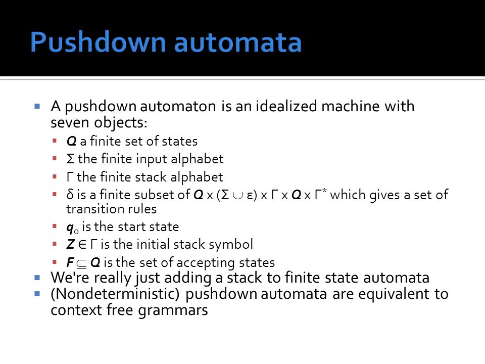
38.  A finite-state automaton is an idealized machine composed of five objects: 1. A finite set I, called the input alphabet, of input symbols 2. A set S of states the automaton can be in 3. A designated state s 0 called the initial state 4. A designed set of states called the set of accepting states 5. A next-state function N: S x I  S that maps a current state with current input to the next state

39.  FSA's are often described with a state transition diagram  The starting state has an arrow  The accepting states are marked with circles  Each rule is represented by a labeled transition arrow  The following FSA represents a vending machine 0¢ 25¢ 75¢ 50¢ $1 $1.25 half-dollar quarter half-dollar quarter half-dollar quarter

40.  Consider this FSA:  We can also describe an FSA using an annotated next-state table  A next-state table gives shows what the transition is for each state for all possible input  An annotated next-state table also marks the initial state and accepting states s0s0 s0s0 s1s1 s1s1 s2s2 s2s2 1 1 0 0 1 0 01  s0s0 s1s1 s0s0 s1s1 s1s1 s2s2  s2s2 s1s1 s0s0

41.  Two states of a finite-state automaton are *- equivalent if any string accepted by the automaton when it starts from one state is accepted when starting from the other  Given an automaton A with eventual-state function N *, we can formally say:  States s and t in A are*-equivalent iff N * (s,w) and N * (t,w) are both accepting states or both not  It turns out that *-equivalence defines an equivalence relation

42.  *-equivalence is hard to demonstrate directly  Instead, we'll focus on equivalence after k or fewer inputs  Given an automaton A with eventual-state function N *, we can formally say:  States s and t in A are k-equivalent iff N * (s,w) and N * (t,w) are both accepting states or both not, for all strings w of length k or less

43.  Keep finding k-equivalence classes for larger and larger values of k  If you ever find that the set of k-equivalence classes is equal to the set of (k+1)-equivalence classes, that is the set of *-equivalence classes  This is known as a fixed point in mathematics  Using the *-equivalence classes, we can build the quotient automaton that is the smallest FSA that accepts a given language  Two equivalent FSA's must have the same quotient automaton (except for labels)

44.  A context free language is one that can be described by a context free grammar  Every regular language is context free, but there are context free languages that are not regular  Classic examples:  Strings of k 0's followed by k 1's  Palindromes made up of a's and b's  Legally nested parentheses  All of these involve counting arbitrary numbers of characters  Regular expressions can't count

45.  A context free grammar G is defined by the 4- tuple G = (V, Σ, R, S)  V is finite set of non-terminals  Σ is a finite set of terminals  R is a finite relation from V to (V  Σ) * which defines the production rules  S is the start symbol

47.  Noam Chomsky is a brilliant linguist who has recently focused mostly on political activism  Remember that a grammar consists of terminals (alphabet symbols), non-terminals, production rules, and a start symbol  He noted that grammars can be divided into four levels in terms of expressiveness:  Type-0 (Unrestricted grammars)  Type-1 (Context sensitive grammars)  Type-2 (Context free grammars)  Type-3 (Regular grammars)

48.  Each grammar has rules for what is a legal production rule  Let α, β, and γ be any combinations of terminals and non- terminals, where γ is non-empty  Unrestricted grammars  α  β (anything to anything)  Context-sensitive grammars  αAβ  αγβ (non-terminal in a particular context to anything)  Context-free grammars  A  γ (a single non-terminal to anything)  Regular grammars  A  a and A  aB (a single non-terminal to a single terminal or a terminal and a single non-terminal on the right side)

49.  Every kind of language has a particular kind of machine associated with it GrammarLanguagesAutomaton Production Rules Examples Type-0 Recursively enumerable Turing machine α  βα  β All languages, any computable functions Type-1 Context- sensitive Linear-bounded non- deterministic Turing machine αAβ  αγβ Most natural human languages Type-2Context-free Non-deterministic pushdown automaton A  γ Most programming languages Type-3RegularFinite state automaton A  a and A  aB Regular expressions

51.  There is no next time!

52.  Final exam  Monday, May 5, 2014  11:00am - 2:00pm