1. ROMS/TOMS TL and ADJ Models: Tools for Generalized Stability Analysis and Data Assimilation Andrew Moore, CU Hernan Arango, Rutgers U Arthur Miller, Bruce Cornuelle, Emanuele Di Lorenzo, Doug Neilson UCSD

2. Major Objective To provide the ocean modeling community with analysis and prediction tools that are available in meteorology and NWP, using a community OGCM (ROMS). To provide the ocean modeling community with analysis and prediction tools that are available in meteorology and NWP, using a community OGCM (ROMS).

3. Overview NL ROMS: NL ROMS: Perturbation: Perturbation:

4. Overview NL ROMS: NL ROMS: TL ROMS: TL ROMS: AD ROMS: AD ROMS: (TL1) (AD)

5. Overview Second TLM: Second TLM: (TL2 ) TL1= Representer Model TL1= Representer Model TL2= Tangent Linear Model TL2= Tangent Linear Model

6. Current Status of TL and AD All advection schemes All advection schemes Most mixing and diffusion schemes Most mixing and diffusion schemes All boundary conditions All boundary conditions Orthogonal curvilinear grids Orthogonal curvilinear grids All equations of state All equations of state Coriolis, pressure gradient, etc. Coriolis, pressure gradient, etc.

7. Generalized Stability Analysis Explore growth of perturbations in the ocean circulation. Explore growth of perturbations in the ocean circulation.

8. Available Drivers (TL1, AD) Singular vectors: Singular vectors: and Eigenmodes of Eigenmodes of Forcing Singular vectors: Forcing Singular vectors: Stochastic optimals: Stochastic optimals: Pseudospectra: Pseudospectra:

9. Two Interpretations Dynamics/sensitivity/stability of flow to naturally occurring perturbations Dynamics/sensitivity/stability of flow to naturally occurring perturbations Dynamics/sensitivity/stability due to error or uncertainties in forecast system Dynamics/sensitivity/stability due to error or uncertainties in forecast system Practical applications: ensemble prediction, adaptive observations, array design... Practical applications: ensemble prediction, adaptive observations, array design...

10. Southern California Bight (SCB) Model grid 1200kmX1000km Model grid 1200kmX1000km 10km resolution, 20 levels 10km resolution, 20 levels Di Lorenzo et al. (2003) Di Lorenzo et al. (2003)

11. SCB Examples

12. Eigenspectrum

13. Eigenmodes (coastally trapped waves)

14. Pseudospectrum Consider Consider Response is proportional to Response is proportional to For a normal system For a normal system For nonnormal system For nonnormal system

15. Pseudospectrum

16. Singular Vectors Consider the initial value problem. Consider the initial value problem. We measure perturbation amplitude as: We measure perturbation amplitude as: Consider perturbation growth factor: Consider perturbation growth factor:

17. Singular Vectors Energy norm, 5 day growth time Energy norm, 5 day growth time

18. Confluence and diffluence

19. SV 1

20. SV 5

21. Boundary sensitivity

22. Seasonal Dependence

23. Forcing Singular Vectors Consider system subject to constant forcing: Consider system subject to constant forcing: Forcing singular vectors are eigenvectors of: Forcing singular vectors are eigenvectors of:

24. Stochastic Optimals Consider system subject to forcing that is stochastic in time: Consider system subject to forcing that is stochastic in time: Assume that: Assume that: Stochastic optimals are eigenvectors of: Stochastic optimals are eigenvectors of:

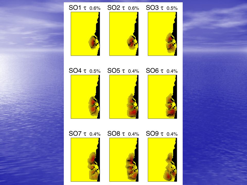
25. Stochastic Optimals (energy norm)

26. Interpretation Optimal forcing for coastally-trapped waves? Optimal forcing for coastally-trapped waves? Optimal forcing for recirculating flow in the lee of Channel Islands? Optimal forcing for recirculating flow in the lee of Channel Islands?

28. Stochastic Optimals (transport norm)

29. Transport Singular Vector

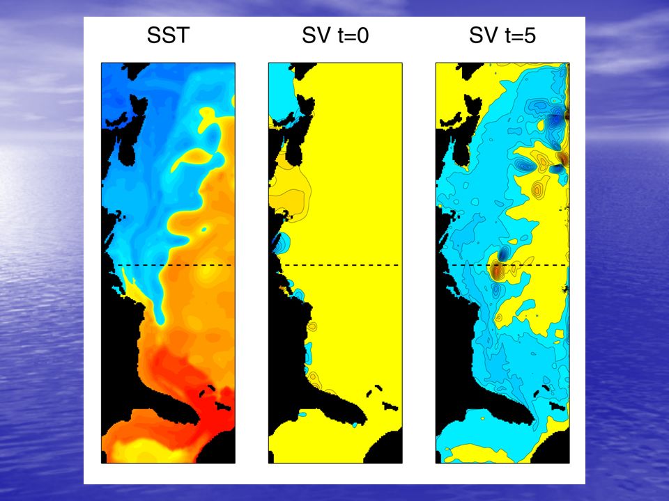
30. North East North Atlantic 10 km resolution 10 km resolution 30 levels in vertical 30 levels in vertical Embedded in a model of N. Atlantic Embedded in a model of N. Atlantic Wilkin, Arango and Haidvogel Wilkin, Arango and Haidvogel

31. SST SV t=0 SV t=5

33. Summary Eigenmodes: natural modes of variability Eigenmodes: natural modes of variability Adjoint eigenmodes: optimal excitations for eigenmodes Adjoint eigenmodes: optimal excitations for eigenmodes Pseudospectra: response of system to forcing at different freqs, and reliability of eigenmode calculations Pseudospectra: response of system to forcing at different freqs, and reliability of eigenmode calculations Singular vectors: stability analysis, ensemble prediction (i.c. errors) Singular vectors: stability analysis, ensemble prediction (i.c. errors)

34. Summary (cont’d) Forcing Singular Vectors: ensemble prediction (model errors) Forcing Singular Vectors: ensemble prediction (model errors) Stochastic optimals: stochastic excitation, ensemble prediction (forcing errors) Stochastic optimals: stochastic excitation, ensemble prediction (forcing errors)

35. Weak Constraint 4DVar NL model: NL model: Initial conditions: Initial conditions: Observations: Observations: For simplicity, assume error-free b.c.s For simplicity, assume error-free b.c.s Cost func: Cost func: Minimize J using indirect representer method Minimize J using indirect representer method (Egbert et al., 1994; Bennett et al, 1997) (Egbert et al., 1994; Bennett et al, 1997)

36. OSU Inverse Ocean Model System (IOM) Chua and Bennett (2001) Chua and Bennett (2001) Provides interface for TL1, TL2 and AD for minimizing J using indirect representer method Provides interface for TL1, TL2 and AD for minimizing J using indirect representer method

37. Initial cond: Initial cond: Outer loop, n Outer loop, n TL2 Inner loop, m Inner loop, m AD TL1 TL2

38. Strong Constraint 4DVar Assume f(t)=0 Assume f(t)=0 Outer loop, n Outer loop, n Inner loop, m Inner loop, m TL1 AD

39. Drivers under development Ensemble prediction (SVs, FSVs, SOs, following NWP) Ensemble prediction (SVs, FSVs, SOs, following NWP) 4D Variational Assimilation (4DVar) 4D Variational Assimilation (4DVar) Greens function assimilation Greens function assimilation IOM interface (IROMS) (NL, TL1, TL2, AD) IOM interface (IROMS) (NL, TL1, TL2, AD)

40. Publications Moore, A.M., H.G Arango, E. Di Lorenzo, B.D. Cornuelle, A.J. Miller and D. Neilson, 2003: A comprehensive ocean prediction and analysis system based on the tangent linear and adjoint of a regional ocean model. Ocean Modelling, Final revisions. Moore, A.M., H.G Arango, E. Di Lorenzo, B.D. Cornuelle, A.J. Miller and D. Neilson, 2003: A comprehensive ocean prediction and analysis system based on the tangent linear and adjoint of a regional ocean model. Ocean Modelling, Final revisions. H.G Arango, Moore, A.M., E. Di Lorenzo, B.D. Cornuelle, A.J. Miller and D. Neilson, 2003: The ROMS tangent linear and adjoint models: A comprehensive ocean prediction and analysis system. Rutgers Tech. Report, In preparation. H.G Arango, Moore, A.M., E. Di Lorenzo, B.D. Cornuelle, A.J. Miller and D. Neilson, 2003: The ROMS tangent linear and adjoint models: A comprehensive ocean prediction and analysis system. Rutgers Tech. Report, In preparation.

41. What next? Complete 4DVar driver Complete 4DVar driver Interface barotropic ROMS to IOM Interface barotropic ROMS to IOM Complete 3D Picard iteration test (TL2) Complete 3D Picard iteration test (TL2) Interface 3D ROMS to IOM Interface 3D ROMS to IOM

42. SCB Examples

43. Confluence and diffluence

44. Boundary sensitivity

45. Stochastic Optimals