Download presentation
Presentation is loading. Please wait.

1
Alcohol consumption and HDI story TotalBeerWineSpiritsOtherHDI Lifetime span Austria13,246,74,11,60,40,75580,119 Finland12,524,592,242,820,310,80079,724 Poland13,254,723,261,5600,71575,976 Russia15,763,650,16,880,340,64467,260 Uganda11,930,5100,1814,520,45353,261 The Human Development Index (HDI) is a composite statistic of life expectancy, education, and income
 is a composite statistic of life expectancy, education, and income")
2
What is a CORRELATION Correlation – statistical procedure to measure & describe the relationship between two variable

3
Do two variables covary? Are two variables dependent or independent of one another? Can one variable be predicted from another? What is a CORRELATION

4
World is full of COVARY

5
The IQ and brain size

6
Pearson's product-moment coefficient

7
.0 to.2 No relationship to very weak association.2 to.4 Weak association.4 to.6 Moderate association.6 to.8 Strong association.8 to 1.0 Very strong to perfect association Interpretation CAUTION!!! Test the null

8
Testing H0

9
Alcohol consumption and HDI story

10
Correlation and causation

11
B causes A (reverse causation) The more firemen fighting a fire, the bigger the fire is observed to be. Therefore firemen cause an increase in the size of a fire. A causes B and B causes A (bidirectional causation) Increased pressure is associated with increased temperature.Therefore pressure causes temperature. Third factor C (the common-causal variable) causes both A and B) Sleeping with one's shoes on is strongly correlated with waking up with a headache. Therefore, sleeping with one's shoes on causes headache. Illogically inferring causation from correlation Coincidence With a decrease in the wearing of hats, there has been an increase in global warming over the same period. Therefore, global warming is caused by people abandoning the practice of wearing hats.
 Increased pressure is associated with increased temperature.Therefore pressure causes temperature. Third factor C (the common-causal variable) causes both A and B) Sleeping with one s shoes on is strongly correlated with waking up with a headache. Therefore, sleeping with one s shoes on causes headache. Illogically inferring causation from correlation Coincidence With a decrease in the wearing of hats, there has been an increase in global warming over the same period. Therefore, global warming is caused by people abandoning the practice of wearing hats..")
12
Church of the Flying Spaghetti Monster

13
Alcohol consumption and HDI story

14
Scatterplot Scatter plot of spousal ages, r = 0.97 Scatter plot of Grip Strength and Arm Strength, r = 0.63

15
Farnsworth favorite game

16
Anscombe’s quartet IIIIIIIV xyxyxyxy 10.08.0410.09.1410.07.468.06.58 8.06.958.08.148.06.778.05.76 13.07.5813.08.7413.012.748.07.71 9.08.819.08.779.07.118.08.84 11.08.3311.09.2611.07.818.08.47 14.09.9614.08.1014.08.848.07.04 6.07.246.06.136.06.088.05.25 4.04.264.03.104.05.3919.012.50 12.010.8412.09.1312.08.158.05.56 7.04.827.07.267.06.428.07.91 5.05.685.04.745.05.738.06.89 PropertyValue Mean of x in each case 9 Variance of x in each case 11 Mean of y in each case 7.50 Variance of y in each case 4.122 or 4.127 Correlation between x and y in each case 0.816

17
Anscombe’s quartet IIIIIIIV xyxyxyxy 10.08.0410.09.1410.07.468.06.58 8.06.958.08.148.06.778.05.76 13.07.5813.08.7413.012.748.07.71 9.08.819.08.779.07.118.08.84 11.08.3311.09.2611.07.818.08.47 14.09.9614.08.1014.08.848.07.04 6.07.246.06.136.06.088.05.25 4.04.264.03.104.05.3919.012.50 12.010.8412.09.1312.08.158.05.56 7.04.827.07.267.06.428.07.91 5.05.685.04.745.05.738.06.89 PropertyValue Mean of x in each case 9 Variance of x in each case 11 Mean of y in each case 7.50 Variance of y in each case 4.122 or 4.127 Correlation between x and y in each case 0.816 CAUTION!!! Check scatterplot

18
Anscombe’s quartet

19
Problems

20
Problems: Outliers r=0,63 r=0,23

21
Problems: Range restriction

22
Coefficient of Determination (r 2 ) CoD = The proportion of variance or change in one variable that can be accounted for by another variable.
 CoD = The proportion of variance or change in one variable that can be accounted for by another variable.")
23
Problems: Range restriction

24
REGRESSION MODELS

25
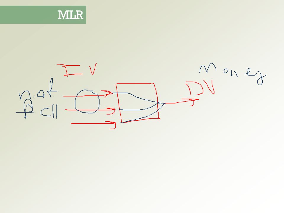
Multiple linear regression (MLR) is a multivariate statistical technique for examining the linear correlations between two or more independent variables (IVs) and a single dependent variable (DV). MLR

27
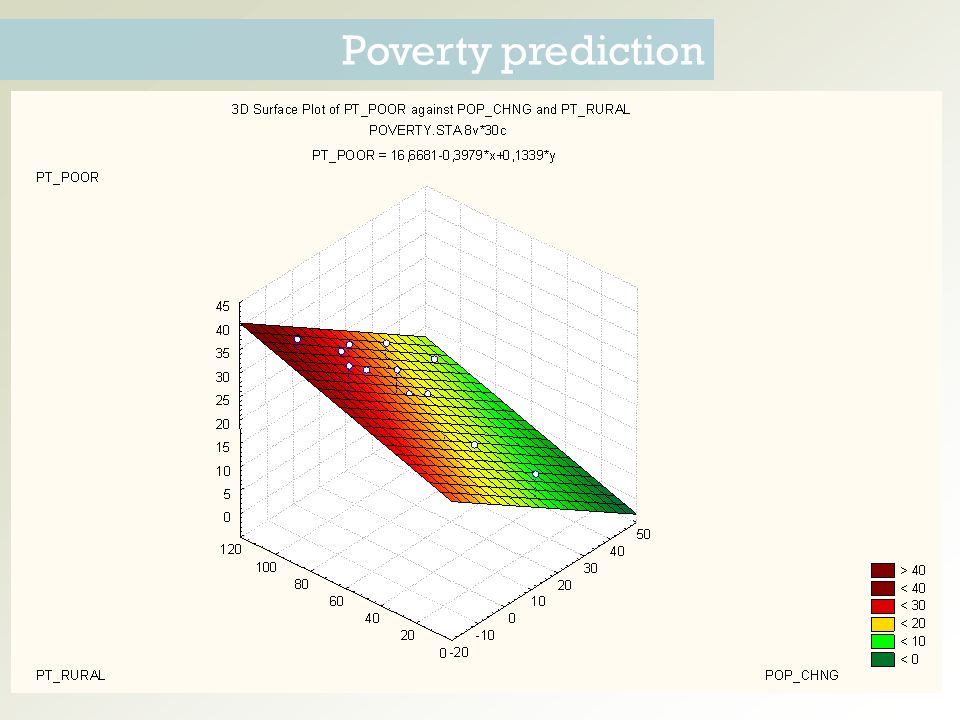
Poverty prediction

28
Name of region Population change in 10 years. No. of persons employed in agriculture Percent of families below poverty level Residential and farm property tax rate Percent residences with telephones Percent rural population Median age Number of African/Americans

29
Level of measurement IVs: MLR involves two or more continuous (interval or ratio) or nominal variables (require recoding into dummy variables) DV: One continuous (interval or ratio) variable Sample size Total N based on ratio of cases to IVs: Min. 5 cases per predictor (5:1) Ideally 20 cases per predictor (20:1) Linearity Are the bivariate relationships linear? Check scatterplots and correlations between the DV (Y) and each of the IVs (Xs) Check for influence of bivariate outlier Multicollinearity Is there multicollinearity between the IVs? (i.e., are they overly correlated e.g., above.7?) Homoscedasticity The variance of the error is constant across observations. Check scatterplots between Y and each of Xs and/or check scatterplot of the residuals (ZRESID) and predicted values (ZPRED) MLR: Pre-analysis assumptions
 Ideally 20 cases per predictor (20:1) Linearity Are the bivariate relationships linear. Check scatterplots and correlations between the DV (Y) and each of the IVs (Xs) Check for influence of bivariate outlier Multicollinearity Is there multicollinearity between the IVs. (i.e., are they overly correlated e.g., above.7 ) Homoscedasticity The variance of the error is constant across observations. Check scatterplots between Y and each of Xs and/or check scatterplot of the residuals (ZRESID) and predicted values (ZPRED) MLR: Pre-analysis assumptions.")
30
MLR: Dummy coding for nominal data

31
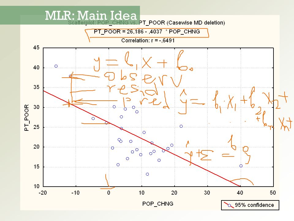
MLR: Main Idea

33
Poverty prediction

35
MLR: Post-analysis assumptions Multivariate outliers Check whether there are influential multivariate outlying cases using Mahalanobis' Distance (MD) & Cook’s D (CD). Normality of residuals Residuals are more likely to be normally distributed if each of the variables normally distributed Check histograms of all variables in an analysis Normally distributed variables will enhance the MLR solution

36
MLR: Post-analysis assumptions

37
Poverty prediction

38
MLR: Types of MLR Direct (or Standard) All IVs are entered simultaneously Hierarchical IVs are entered in steps, i.e., some before others Interpret R 2 change Forward The software enters IVs one by one until there are no more significant IVs to be entered Backward The software removes IVs one to one until there are no more non-significant IVs to removed Stepwise A combination of Forward and Backward MLR
 All IVs are entered simultaneously Hierarchical IVs are entered in steps, i.e., some before others Interpret R 2 change Forward The software enters IVs one by one until there are no more significant IVs to be entered Backward The software removes IVs one to one until there are no more non-significant IVs to removed Stepwise A combination of Forward and Backward MLR")
39
MLR: TOTAL 1.Conceptualise the model 2.Recode predictors (if necessary) 3.Check assumptions 4.Choose the type of MLR 5.Interpret statistical output and meaning of results. 6.Depict the relationships in a path diagram or Venn diagram 7.Regression equation: If relevant and useful, interpret Y-intercept and write a regression equation for predicting Y

Similar presentations