2.  Combines linear regression and ANOVA  Can be used to compare g treatments, after controlling for quantitative factor believed to be related to response (e.g. pre-treatment score)  Can be used to compare regression equations among g groups (e.g. common slopes and/or intercepts)

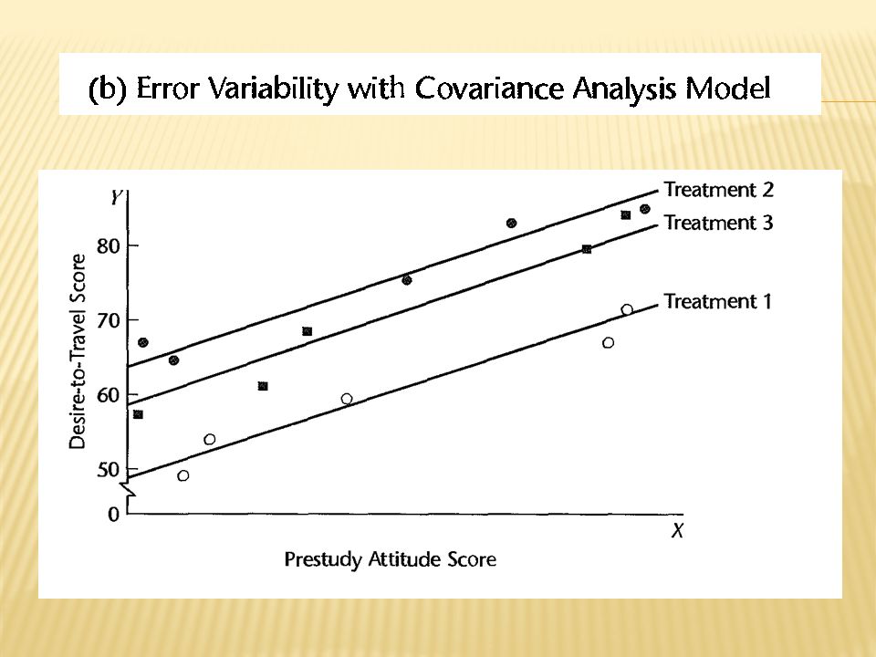
7. 3. The covariate does not affect the differences among the means of the groups (treatments). If differences among the group means were reduced when the dependent variable is adjusted for the covariate, the test for equality of group means would be less powerful.  Assumption 3 can be checked by performing an ANOVA on the covariate.

8. we wish to compare three methods of teaching language. Three classes are available, and we assign a class to each of the teaching methods. The students are free to sign up for any one of the three classes and are therefore not randomly assigned. One of the classes may end up with a disproportionate share of the best students, in which case we cannot claim that teaching methods have produced a significant difference in final grades. However, we can use previous grades or other measures of performance as covariates and then compare the students’ adjusted scores for the three methods.

10. We assume:  Z is less than full rank as in overparameterized ANOVA models and  X is full-rank as in regression models  and  Parameter estimation:

13.  The test statistic is given by:

16.  The test statistic is:  which is distributed as F[k-1, k(n-2)] when is true.

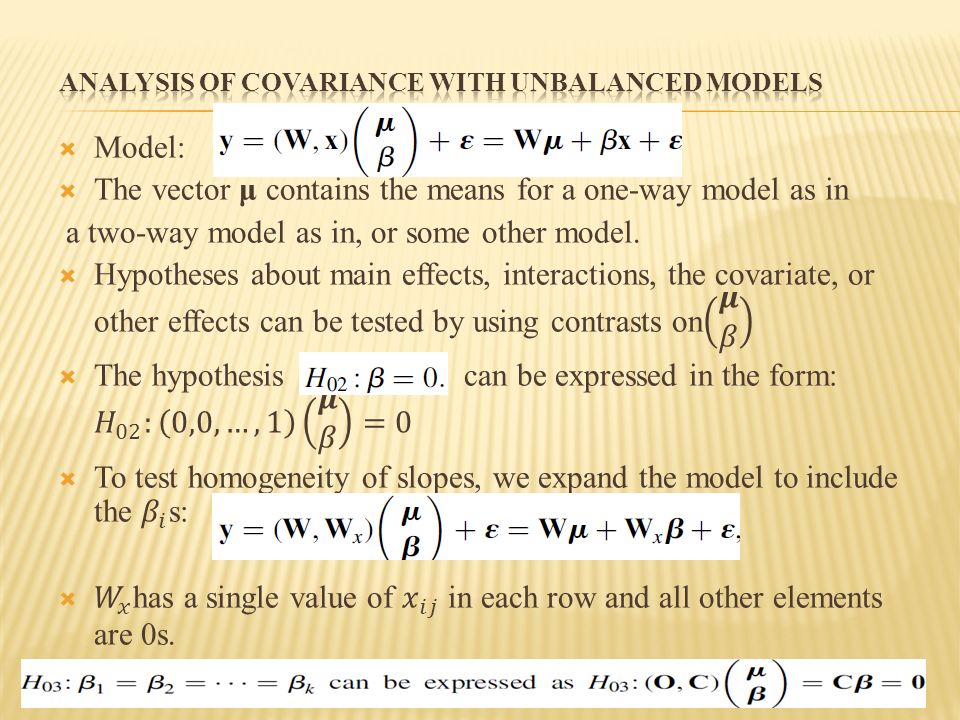
18.  Model:  Estimation:

19.  Test for main effects and interaction  Test for Slope Vector  Test for Homogeneity of Slope Vectors: that the k regression planes (for the k treatments) are parallel.

21.  Blocking – may be the best alternative:  Because it doesn’t have the special assumptions of ANCOVA  Because it can capture non-linear relationships between CV and DV where ANCOVA only deals with linear relationships.

22. GLM Univariate

23. data glue; input FormulationStrengthThickness; datalines; 146.513 145.914 149.812 146.112 144.314 248.712 249.010 250.111 248.512 245.214 346.315 347.114 348.911 348.211 350.310 444.716 443.015 451.010 448.112 446.811 ; run; proc glm; class formulation; model strength = thickness formulation / solution ; lsmeans formulation / stderr pdiff; run;

24. Stat > ANOVA > General Linear Model … > Responses: Strength > Model: Formulation > Covariates: Thickness > Options: Adjusted (Type III) Sums of Squares Factor Plots… > Main Effects Plot > Formulation

25. 23-25 > glue <- read.table("glue.txt",header=TRUE) > glue$Formulation <- as.factor(glue$Formulation) > # fit linear models: full, thickness only, formulation only > full.lm <- lm(Strength ~ Formulation + Thickness, data=glue) > thick.lm <- lm(Strength ~ Thickness, data=glue) > formu.lm <- lm(Strength ~ Formulation, data=glue) > > anova(thick.lm,full.lm) Analysis of Variance Table Model 1: Strength ~ Thickness Model 2: Strength ~ Formulation + Thickness Res.Df RSS Df Sum of Sq F Pr(>F) 1 18 27.2563 2 15 24.4468 3 2.8095 0.5746 0.6405 > anova(formu.lm,full.lm) Analysis of Variance Table Model 1: Strength ~ Formulation Model 2: Strength ~ Formulation + Thickness Res.Df RSS Df Sum of Sq F Pr(>F) 1 16 77.648 2 15 24.447 1 53.201 32.643 4.105e-05 *** Test for Formulation differences Test for significance of Thickness

26. 23-26 > summary(full.lm) Call: lm(formula = Strength ~ Formulation + Thickness, data = glue) Residuals: Min 1Q Median 3Q Max -1.6380 -1.0398 0.1873 0.6966 2.3255 Coefficients: Estimate Std. Error t value Pr(>|t|) (Intercept) 58.92788 2.24551 26.243 5.97e-14 *** Formulation2 0.63466 0.83193 0.763 0.457 Formulation3 0.87644 0.81840 1.071 0.301 Formulation4 0.00911 0.80810 0.011 0.991 Thickness -0.95445 0.16706 -5.713 4.11e-05 *** > summary(thick.lm) Call: lm(formula = Strength ~ Thickness, data = glue) Residuals: Min 1Q Median 3Q Max -2.0813 -0.7324 0.1274 0.9090 1.9230 Coefficients: Estimate Std. Error t value Pr(>|t|) (Intercept) 59.9294 1.9504 30.726 < 2e-16 *** Thickness -1.0044 0.1551 -6.476 4.32e-06 *** Residual standard error: 1.231 on 18 degrees of freedom Multiple R-Squared: 0.6997, Adjusted R-squared: 0.683 F-statistic: 41.94 on 1 and 18 DF, p-value: 4.317e-06 Full model (can be refined by omitting formulation) Reduced model (formulation omitted)