1. Non-Baryonic Dark Matter in Cosmology
Antonino Del Popolo
Department of Physics and Astronomy
University of Catania, Italy
IX Mexican School on Gravitation and Mathematical Physics
"Cosmology for the XXI Century: Inflation, Dark Matter and Dark Energy"
Puerto Vallarta, Jalisco, Mexico, December 3-7, 2012 1 1

2. LECTURE 2 The distribution of Dark Matter in galaxies and clusters

3. Stellar Disks SPIRALS Ropt=3.2RD M33 - outer disk truncated,
very smooth structure
NGC exponential disk
goes for at least 10 scale-
lengths
Ropt=3.2RD
scale
radius
Bland-Hawthorn et al 2005
Ferguson et al 2003 3 3

4. Gas surface densities GAS DISTRIBUTION HI Flattish radial distribution4
Gas surface densities
GAS DISTRIBUTION HI
Flattish radial distribution
Deficiency in centre
CO and H2
Roughly exponential
Negligible mass
Wong & Blitz (2002)
Berkeley-Illinois-. Maryland Association (BIMA) Array with 30 GHz receivers. 4 4

5. Circular velocities from spectroscopy 5
Circular velocities from spectroscopy
- Optical emission lines (H, Na)
- Neutral hydrogen (HI)-carbon monoxide (CO)
HI -> 21 cm
CO -> mm -> range [e.g., GHz for 12CO
(J = 1 -0) line, GHz for J =(2 -1)
Tracer angular resolution spectral resolution
HI 7" … 30" 2 … 10 km s-1
CO 1.5" … 8" 2 … 10 km s-1
H, … 0.5" … 1.5" … 30 km s-1 5 5

6. 6
ROTATION CURVES(RCs)
A RC is obtained calculating the rotational velocity of a tracer (e.g. stars, gas) along the
length of a galaxy by measuring their Doppler shifts, and then plotting this quantity versus
their respective distance away from the centers
Tracing the intensity-weighted velocities
I(v)= intensity profile at a given radius as a function of the radial velocity.
The rotation velocity is then given by
i= inclination angle
Vsys= systemic velocity of the galaxy. .
EXAMPLE OF HIGH QUALITY RC
Optical
resolution: 2”, i.e.
RD/30-RD/10
Radio Interferometers:
10” 6 6

7. - Bosma 1981: HI RCs for 25 galaxies well extended beyond7
Extended HI kinematics traces dark matter -
Light (SDSS)
HI velocity field
NGC 5055
Ropt
Bosma 1981:
HI RCs for 25
galaxies well
extended beyond
the optical radio
(e.g. NGC 5055)
SDSS
Bosma, 1981
GALEX
Radius (kpc)
Bosma 1979
The mass discrepancy emerges as a disagreement between light and mass distributions 7 7

8. From data to mass models8
Rotation curve analysis
From data to mass models
observations
model
Vtot2 = Vhalo2 + Vdisk*2 + VHI2+(Vb2)
Model parameters
from I-band photometry
from HI observations
different choices for the DM halo density
Dark halos with cusps (NFW, Einasto)
Dark halos with constant density cores (Burkert)
Model has three free parameters: disk mass, halo central density and core radius (halo length-scale)
Obtained by best fitting method. 8 8

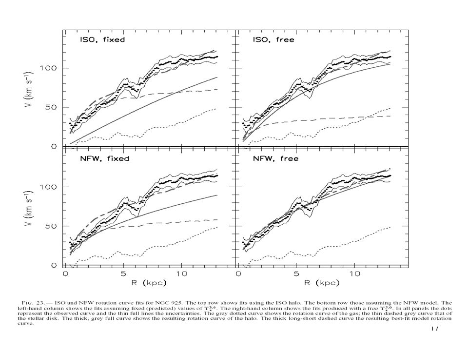
9. = rs/(1+r/rs)(1+(r/rs)2) NFW r = rs/(r/rs)(1+r/rs)2 Moore
Gentile et al. 2004, 2007
rotational curves of spiral galaxies decomposed into their stellar, gaseous and dark matter components.
fit to the inferred density distribution
with various models
models with a constant density core are preferred.
Burkert: with a DM core
= rs/(1+r/rs)(1+(r/rs)2)
NFW
r = rs/(r/rs)(1+r/rs)2
Moore
r = rs/(r/rs)1.5(1+(r/rs)1.5)
HI-scaling, with a cst factor
MOND, without DM
Mass models for the galaxy Eso 116-G12. Solid line: best fitting model,
long-dashed line: DM halo; dotted: stellar; dashed: gaseous disc.
1kpc corresponds to 13.4 arcsec. Below: residuals: (Vobs-Vmodel) 9

10. Maximum disk fit: NGC 2976
Significant radial motions in inner 30” (blue)
Rotation velocity derived from combined CO and Hα velocity field
Radial velocity
Systemic velocity

11. HI H2

12. An upper limit on the dark matter rotation curve (and also the slope of the density profile) can
be found if the disk mass is zero (minimum disk or maximul halo), and a lower limit to the dark
matter rotation curve and density profile slope is obtained for a maximum disk. In general, for
galaxies of normal surface brightness, the minimum disk solution is physically unrealistic and the
actual mass distribution is likely to be closer to the maximum disk case.
stars

13. To reveal the shape of the density profile of DM halo, we need to remove the rotational velocities contributed by the baryonic components of the galaxy. The rotation curve of the dark matter halo is defined by
The lower limit to the DM density profile is obtained by maximizing the rotation curve contribution from the stellar disk. The maximum
possible stellar rotation curve is set by scaling up the mass-to-light ratio of the stellar disk until the criterion
is no longer met at every point of the rotation curve.This requirement sets maximum disk mass-to-light ratios M/Lk
Maximal disk
dark halo

14. Maximum Disk Fit No cusp! Even with no disk, dark Maximal disk M*/LK =
halo density profile is
r(r) = 1.2 r ± 0.09 M/pc3
Maximal disk M*/LK =
0.19 M/L,K
After subtracting stellar
disk, dark halo structure is
r(r) = 0.1 r ± 0.12M/pc3
No cusp!

15. MASS MODELLING RESULTS
highest luminosities
lowest luminosities
halo
disk
disk
halo
halo
disk
Smaller galaxies are denser and have a higher proportion of dark matter.
core radius
halo central density
luminosity
fraction of DM
Read & Trentham 2005 15 15

16. The distribution of DM around spirals
1616
The distribution of DM around spirals
Using individual galaxies de Blok+ 2008  Kuzio de Naray , Oh+  2008,
A detailed investigation: high quality data and model independent analysis
Survey of HI emission in 34 nearby galaxies obtained using the NRAO Very Large Array (VLA).
High spectral (≤5.2 km/s) and spatial (~6'') resolution
Distances 2 < D < 15 Mpc
Masses M HI (0.01 to 14 × 109 M ☉), absolute luminosities MB (–11.5 to –21.7 mag)
de Blok et al. (2008): galaxies having MB < −19 -> NFW profile or an PI profile statistically fit equally well
MB > −19 the core dominated PI model fits significantly better than the NFW model. 16

18. 1818
DDO 47
Oh et al. (2010)
THINGS dwarfs
General results from several samples including THINGS, HI survey of uniform and high quality data
- Non-circular motions are small.
- No DM halo elongation
- ISO halos often preferred over NFW
Tri-axiality and non-circular motions cannot explain
the CDM/NFW cusp/core discrepancy 18 18

19. SPIRALS: WHAT WE KNOW
MORE PROPORTION OF DARK MATTER IN SMALLER SYSTEMS
MASS PROFILE AT LARGER RADII COMPATIBLE WITH NFW
DARK HALO DENSITY SHOWS A CENTRAL CORE OF SIZE 2 RD

20. Assuming radially constant stellar mass to light ratio
2020
ELLIPTICALS
The Stellar Spheroid
Surface brightness follows a Sersic (de Vaucouleurs) law
Re : the effective radius, n Sersic index (light concentration)
By deprojecting I(R) we obtain the luminosity density j(r):
for n=4
Relatively featureless spheroidal galaxies
Assuming radially constant stellar mass to light ratio
ESO
Sersic profile
V (triangles) and I-band (boxes)
Surface brightness profiles
The solid lines are
the best-fit Sersic profiles
Jerjen & Rejkuba 2001
Central surface brightness 20 20

21. -Rotation is not always negligible
2121
Kinematics of ellipticals: Jeans modelling of radial, projected and aperture velocity dispersions
measure I(R), σP (R)
derive Mh(r), Msph(r)
radial V ϬP
projected (or line of sight)
aperture
projected
luminosity
-Rotation is not always negligible
-Ϭr (R) is a direct probe of grav potential but it is not observable
-ϬP (R) is observable when individual star measures are available
-ϬAP is the standard observable
The projected velocity dispersion, σp, is the quantity measured at the telescope either by comparing the galaxy absorption spectrum to broadened stellar templates or by measuring the galaxy velocity dispersion in different radial bins, depending on the program. Different observational effects may be taken into account in the analysis, with some discussion presented in Chapter 3. Since it is difficult to compile the necessary radial velocities in one cluster, itis common to “stack” the results from many similar clusters.
SAURON data of N 2974
When observed through an aperture of finite size, the projected
velocity dispersion profile, σp is weighted on the brightness
profile I(R). 21

22. Modelling Ellipticals
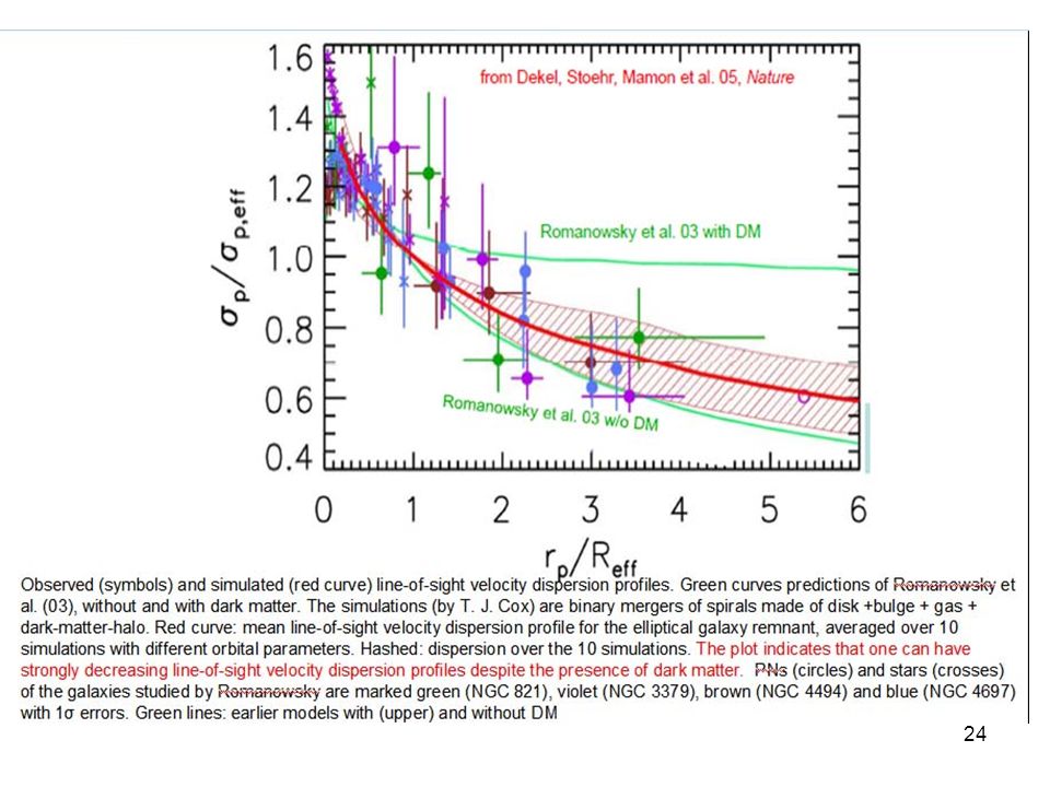
Measure the light profile= stellar mass profile (M*/L)-1
Derive the total mass M(r) profile from
-Virial theorem
-Dispersion velocities of kinematical tracers (e.g., stars, Planetary Nebulas)
Disentangle M(r) into its dark and the stellar components. In ellipticals gravity is balanced by pressure gradients -> Jeans Equation
Difficulties in inferring the presence of dark matter halos in ellipticals:
the velocity dispersions of the usual kinematical tracer, stars, can only be measured out to 2Re.
Mass/anisotropy degeneracy: For a given ρ(r), σr(r), two unknown remains: M(r), and β(r) and one cannot solve Jeans equation for both, unless one assumes no rotation and makes use of the 4th order moment (kurtosis) of the velocity distribution (Lokas & Mamon 2003).
(One of the first studies Romanowsky et al > a dearth of DM in E)
Spherical Symmetry;
Non-rotating system
L(r ) luminosity density
Velocity dispersion anisotropy or
This plot compares observed (symbols) and simulated (red curve) line-of-sight velocity dispersion profiles. r_p = projected radius. R_eff = effective radius (within which half the projected light lies). sigma_p = line-of-sight velocity dispersion. sigma_p,eff = line-of- sight velocity dispersion at projected radius r_p=R_eff. The green curves were predictions of Romanowsky et al. (03, Science), without and with dark matter. The simulations (by T. J. Cox) are binary mergers of spirals made of disk+bulge+gas+dark-matter- halo. The red curve is the mean line-of-sight velocity dispersion profile for the elliptical galaxy remnant, averaged over 10 simulations with different orbital parameters. The hashed region shows the dispersion over the 10 simulations. The plot indicates that one can have strongly decreasing line-of-sight velocity dispersion profiles despite the presence of dark matter.
The merger remnants are viewed from three orthogonal directions and the 60 profiles are stacked such that the stellar curves (“all”) match at Reff.
Colors and line types are as in Fig. 1. The < 3 Gyr “young” stars may mimic the observed PNs. The 1σ scatter is marked by shaded or hashed areas or a thick bar. The galaxies are marked green (821), violet (3379), brown (4494) and blue (4697) with 1σ errors; PNs (circles) and stars (crosses). The surface densities shown for 3 galaxies almost coincide with the simulated profile. Green lines refer to the earlier models with (upper) and without DM
-X-ray properties of the emitting hot gas
-Combining weak and strong lensing data

23. Jeans modelling of PN data with a stellar spheroid + NFW dark halo
2323
slide1
Jeans modelling using PN *
Pseudo inversion mass model
Napolitano et al. (2011)
NGC 4374
Napolitano et al. (2011)
ML05: Mamon & Lokas 2005
Ellipticals have big DM halos (usually cuspy profiles, sometime cored
Jeans modelling of PN data with a stellar spheroid + NFW dark halo
e.g.
This plot compares observed (symbols) and simulated (red curve) line-of-sight velocity dispersion profiles. r_p = projected radius. R_eff = effective radius (within which half the projected light lies). sigma_p = line-of-sight velocity dispersion. sigma_p,eff = line-of-sight velocity dispersion at projected radius r_p=R_eff. The green curves were predictions of Romanowsky et al. (03, Science), without and with dark matter. The simulations (by T. J. Cox) are binary mergers of spirals made of disk+bulge+gas+dark- matter-halo. The red curve is the mean line-of-sight velocity dispersion profile for the elliptical galaxy remnant, averaged over 10 simulations with different orbital parameters. The hashed region shows the dispersion over the 10 simulations. The plot indicates that one can have strongly decreasing line-of-sight velocity dispersion profiles despite the presence of dark matter.
WMAP1
Multicomponent model
(0) Parametrized mass profile, e.g. NFW 23

25. Exercise: Virial theorem, Planetary Nebulae -> M/L
Example: For planetary nebulae around NGC1399, the average rotation Vr≈300kms-1, and the velocity dispersion σ≈400kms-1 at 25kpc radius. Assumed that the random speed are equal in all directions and the galaxy is roughly spherical, find the total mass within 25kpc of the center. Given that NGC1399 has MV=-21.7, show that M/L~80.
PN: low-mass stars exhaust their nuclear fuel; core’s ultraviolet radiation ionizes outer gas; strongly in emission
lines, e.g., [OIII]5007A.

26. Solution:
Virial theorem

27. Dark-Luminous mass decomposition of dispersion velocities
2727
Dark-Luminous mass decomposition of dispersion velocities 1
Assumed Isotropy Three components: DM, stars (Sersic), Black Holes Naive superposition of Sersic models for the stellar mass component of L=L* elliptical galaxies with hot gas (from X rays) and central black hole (from the Magorrian relation), plus Dark Matter models: NFW; Jing & Suto; Einasto (Nav04). No adiabatic contraction.
Mamon & Łokas 05
This plot indicates that while dark matter dominates
outside of a few Re, the stellar component dominates inside
Re. Therefore, it is difficult to measure the amount of dark
matter in the inner regions of ellipticals.
The 6 plots show a naive superposition of Sersic models for the stellar mass component of L=L* elliptical galaxies with hot gas (from X rays) and central black hole (from the magorrian relation), plus Dark Matter models (NFW = Navarro, Frenk & White 96 [with a 1/r central density cusp]; JS-1.5 = Jing & Suto 00 [with a 1/r^{3/2} central cusp]; Nav04 = Einasto model (Navarro et al which fits best the “LCDM” halos in dissipationless cosmological simulations). There is no adiabatic contraction of the dark matter in these models. This plot indicates that while dark matter dominates outside of a few R_e = R_eff [= half- projected-light radius], the stellar component dominates inside R_e. Therefore, it is difficult to measure the amount of dark matter in the inner regions of ellipticals.
The spheroid determines the velocity dispersion Stars dominate inside Re Dark matter profile “unresolved” 27 27

28. Gravitational Lensing formalism
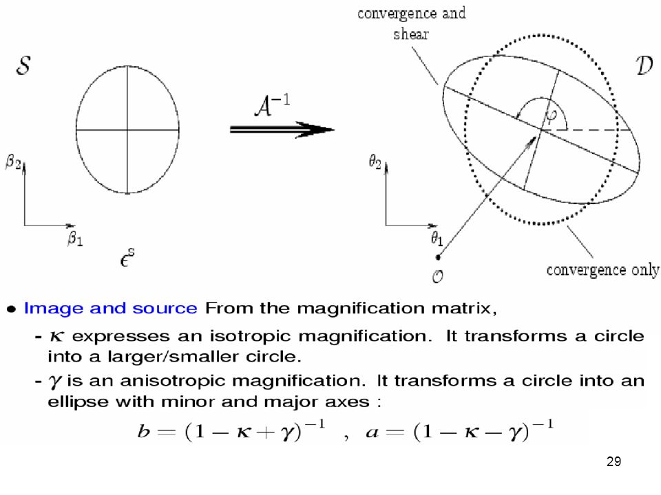
Deflection angle
The deflection angle relates a point in the source plane to its image(s)
in the image plane through the lens equation
Deflection potential
Convergence
• For a lens of 1 solar mass located at 1 AU and a source a 1 kpc -> Theta_E= arc-second
• For a lens of 1011 solar masses located at 100kpc and a source at 300 kpc Theta_E= 1 arc-second
• For a lens of 1015 solar masses located at 1Gpc and a source at 3 Gpc Theta_E= 30 arc-second (sensitive to cosmological parameters)
-- Typical value: cluster of galaxies of 1015 masses at 1Gpc and sources at 2 Gpc :
- Sigma_crit= 0.5 g/cm2
Surface mass density
Angular radius and mass of
an Einstein ring
angle between
and x
Jacobian  between
the unlensed and lensed
coordinate systems
z= los coordinate
ξ=vector in the
plane of sky
The term involving the convergence magnifies the image by increasing its
size while conserving surface brightness. The term involving the shear
stretches the image tangentially around the lens

30. Definitions of Ellipticity
where
Image ellipticity unbaiased
estimate of shear
Source orientation
Isotropically istributed
->

31. Weak lensing mass reconstruction*
In Fourier space
Eq. * , convolution
Inverting

32. n

33. Exercise: calculate the mass enclosed in an Einstein ring
Lens equation
for
Being
This is nearly true for the elliptical case as well.
For multiple imaging systems (those that aren’t necessarily lensed into Einstein
rings) the typical separation between images is ∼ 2θE.

35. Mass profiles from weak lensing
3535
Mass profiles from weak lensing
Lensing equation for the observed tangential shear
e.g. Schneider,1996
Shear= Tangential term+curl
For a circularly symmetric lens the curl vanish
and the tangential part is
Background round galaxy (of semi axis a/b = 1), whose line of the sight passes at distance R from the center of a lensing galaxy ->will be seen with a (very small) ellipticity a/b - 1 =10-3. Averaging on a very large number of objects
we observe a tangential shear γt. The lens equation relates γt with the distribution of matter around the lensing galaxy
Projected mass density of the
object distorting the galaxy
Mean projected mass
density interior
to the radius R
The DM distribution is obtained by fitting the observed
shear with a chosen density profile with 2 free parameters. 35

36. MODELLING WEAK LENSING SIGNALS
Lenses: isolated galaxies, sources: SDSS galaxies
NFW
0.1
0.1
tar
tar
Mandelbaum et al 2009
HALOS EXTEND OUT
TO VIRIAL RADII
Using the previous method, Mandelbaum et al. (2006, 2009) measured
the shear around galaxies of different luminosities out to kpc
reaching out the virial radius, although with a not negligible observational
uncertainty. Both NFW and Burkert halo profiles agree with data.

37. OUTER DM HALOS: NFW/BURKERT PROFILE FIT THEM EQUALLY WELL
Donato et al 2009
NFW
Tangential shear measurements from Hoekstra et al. (2005) as a function of projected distance from the lens in five
R-band luminosity bins. In this sample, the lenses are at a mean redshift z ∼ 0.32 and the background sources are,
in practice, at z=∞. The solid (dashed) magenta line indicates the Burkert (NFW) model fit to the data. At low luminosities they agree.

38. Weak and strong lensing
strong lensing measures the total mass inside the Einstein ring
Sloan Lens ACS (SLACS): (Gavazzi et al. 2007)
Strong lensing data of 22 massive
SLACS galaxies modeled as a
sum of stellar component
(de Vaucoulers) + DM
halo (NFW)
AN EINSTEIN RING AT Reinst IMPLIES THERE
A CRITICAL SURFACE DENSITY:
D = ,
Shear profile for the best DM + de Vaucouleurs profile.
The thickness of the total mass curve codes for the 1 sigma uncertainty around the total shear profile. Uncertainties are very small below 10 kpc because of strong lensing data not shown here. The transition between star and DM-dominated mass profile occurs close to the mean effective radius (yellow arrow). The total density profile is close to isothermal over ∼ 2 decades in radius..
average total
mass density
profile
M3D ( 38

39. Strong lensing and galaxy kinematics
Koopmans, 2006
Assume
Fit
γ= logarithmic slope
Koopmans et al. (2006): joint gravitational lensing and stellar-dynamical analysis of a subsample of 15 massive field early-type galaxies from SLACS Survey. Galaxies have remarkably homogeneous inner mass density profiles (ρtot α r−2). Stellar Spheroid mass accounts for most of the total mass inside Re. The figure shows the logarithmic density slope of Slacs lens galaxies as a function of (normalized) Einstein radius.
Inside REinst the total (spheroid + dark halo) mass increase proportionally with radius
Inside REinst the total the fraction of dark matter is small
Inferred dark matter mass fraction inside the
Einstein radius, assuming a constant stellar
M/LB as a function of E/S0 velocity
dispersion
SIE: Singular Isothermal Ellipsoid model

40. Mass Profiles from X-ray
Nagino & Matsushita 2009
gravitational mass profiles of 22 early-type galaxies observed with XMM-Newton and Chandra.
Temperature
Integrated mass profile (Mʘ)
Density
Colors: individual galaxies. Solid lines best-fit function.
M/L profile
NO DM
R/re
Hydrostatic Equilibrium
Summary of M/L ratio of 19 of the 22 galaxies (only two groups) 40

41. ELLIPTICALS: WHAT WE KNOW
SMALL AMOUNT OF DM INSIDE RE
MASS PROFILE COMPATIBLE WITH NFW AND BURKERT?
DARK MATTER DIRECTLY TRACED OUT TO RVIR

42. dSphs

43. Dwarf spheroidals: basic properties
The smallest objects in the Universe, benchmark for theory
Discovery of ultra-faint MW satellites (e.g. Belokurov et a. 2007), extends the range of dSph structural parameters:
1 order of magnitude in radius and 3 in luminosity
1. Apparently in equilibrium
2. Small number of stars
3. No dynamically significant gas
dSph show large Mgrav/L
(10-100)
DM content makes them interesting
Luminosities and sizes of
Globular Clusters and dSph are different
Gilmore et al 2009

44. Kinematics of dSph
1983: Aaronson measured velocity dispersion of Draco based on observations of 3
carbon stars - M/L ~ 30
1997: First dispersion velocity profile of Fornax (Mateo)
2000+: Dispersion profiles of all dSphs measured using multi-object spectrographs
Instruments: AF2/WYFFOS (WHT, La Palma); FLAMES (VLT); GMOS (Gemini); DEIMOS (Keck); MIKE (Magellan)
2010: full radial coverage in each dSph, with stars per galaxy
STELLAR SPHEROID

45. Dispersion velocity profiles
STELLAR SPHEROID
CORED HALO +
STELLAR SPH
Similarity of profiles obtained by different groups with different instruments on different
telescopes is re-assuring.
Star by star comparisons also confirm that (a) individual velocities and estimated errors are correct
and (b) velocity distributions are not strongly affected by unresolved binaries
Dotted curves show mass-follows-light profiles
Wilkinson et al 2009
dSph dispersion profiles generally remain flat to large radii

46. simulations-> Ursa Minor dSph would survive for less
Degeneracy between DM mass profile and velocity anisotropy
Dispersion velocity profiles remain generally flat to large radius
Cored and cusped halos with orbit anisotropy fit dispersion profiles equally well
Walker et al 2009
Isothermal…
Power law ---
HOWEVER
Gilmore et al. (2007) favor a
cored DM profile
Kleyna et al. (2003): N-body
simulations-> Ursa Minor
dSph would survive for less
than 1 Gyr if the DM core
were cusped.
Magorrian (2003):
α= 0.55(+0.37, -0.33)
for the Draco dSph.
σ(R) km/s 46

47. Mass profiles of dSphs Results point to cored distributions
In a collisionless equilibrium systems, Jeans equation relates kinematics, light and underlying mass distribution
Make assumptions on the velocity anisotropy and then fit the dispersion profile-> DM mass distribution
The surface brightness profiles are typically fit by a Plummer distribution (Plummer 1915)
Rb=stellar scale length
PLUMMER PROFILE
Gilmore et al 2007
Results point to cored distributions 47 47

48. DSPH: WHAT WE KNOW
PROVE THE EXISTENCE OF DM HALOS OF 1010 MSUN AND ρ0 =10-21 g/cm3
DOMINATED BY DARK MATTER AT ANY RADIUS
MASS PROFILE CONSISTENT WITH BURKERT PROFILE
HINTS FOR THE PRESENCE OF A DENSITY CORE

49. Galaxy Clusters
Half of all galaxies are in clusters (higher density; more Es and S0; mass > few times ) or groups (less dense; more Sp and Irr; less than 1014Msun)
100s to 1000s of gravitationally bound galaxies
Typically ~few Mpc across
Central Mpc contains 50 to 100 luminous galaxies (L > 2 x 1010 Lsun)
Distribution of galaxies falls ar r ¼ (like surface brightness of elliptical galaxies)
Coma Cluster 49

50. Measuring DM content in clusters
Gravitational lensing: measure mass without regard to the dynamical state of the cluster. Cannot distinguish between light and dark mass components, another mass tracer is needed to disentangle luminous from dark matter (typical structures observed in the strong lensing regime are radial arcs, located in positions corresponding to the local derivative of the cluster mass density profile, and tangential arcs, the position of which is determined by the projected mass density interior to the arc).
X-Ray emission of ICM:
-Measuring rho(r) and T(r) -> Mass distribution of the cluster.
-Technique really only sensitive to the total mass (unable to disentangle luminous from DM)
- Previous concern dismissed because clusters MDM dominated (not totally true: BCG may be significant contributor)
Dynamics
- cluster galaxies (or stars of the BCG) as tracers of the potential.
Osipkov-Merrit parameterization of the anisotropy
The projected velocity dispersion, σp, is the quantity measured at the telescope either by comparing the BCG absorption spectrum to broadened stellar templates or by measuring the galaxy velocity dispersion in different radial bins, depending on the program. Since it is difficult to compile the necessary radial velocities in one cluster, it is common to “stack” the results from many similar clusters.

51. the gas density and temperature.
Figures illustrating the basic observables and results typical for X-ray analyses of cluster mass distributions. Typically, the X-ray
image is split up into a series of circular, concentric annuli, with the spectrum of each annulus compared to a plasma model to infer
the gas density and temperature.
Top Left.Chandra ACIS image of Abell Top Right.Radial gas density profile of Abell 2029 (large circles) fit to several standard
parameterizations. This parameterized fit is then fed into equation for M(r), along with the temperature profile to calculate the enclosed
mass profile. Bottom Left. The radial temperature profile of Abell 2029, again fit to a standard paramaterization to facilitate the
hydrostatic equilibrium analysis. Bottom Right. Total enclosed cluster mass profile. The open circles are the data points and the
lines are .ts to the data, with the NFWprofile being a very good fit.
The upside down triangles show the contribution from the cluster gas mass. Note that the bright yellow band shows the possible
contribution from the cluster BCG,illustrating the need for an additional technique to account for and disentangle this important
mass component in order to understand the dark matter density pro.le. This .gure has been reproduced from Lewis et al. (2002, 2003).
Typically, the X-ray image is split up into a series of circular, concentric annuli, with the spectrum of each annulus compared to a plasma model to infer the gas density and temperature. Attempts are often made to deproject the data using an “onion peeling” technique (Buote, 2000). Then, parameterized models are .t to the gas density and temperature pro.le so that the derivatives in Equation 1.16 are tractable. In this way, an enclosed mass pro.le is calculated and compared to expectations from CDM (see Figure for an illustration).

52. Mass profiles from XMM-Newton
Pointecouteau, Arnaud, and Pratt (2005)
XMM-Newton
Scaled mass profiles of all clusters. The mass is scaled to M200, and the radius to R200, both values being derived from the best
fitting NFWmodel. The solid black line corresponds to the mean scaled NFWprofile and the two dashed lines are the associated
standard deviation.

53. Limits of X-ray mass determination
X-ray data alone have difficulties in constraining the mass distribution, especially in the central regions, since relaxed clusters tend to have “cooling flows”, and in these clusters X-ray emission is often disturbed and the assumption of hydrostatic equilibrium is questionable (see Arabadjis, Bautz & Arabadjis 2004).
X-ray analyses, ALONE, cannot disentangle the DM and baryonic components
X-ray temperature measurements are carried out from 500 kpc (Bradˇac et al. 2008) to 50 kpc. Determination of temperature at smaller radia are limited by instrumental resolution or substructure (Schmidt & Allen 2007).
Complicated to take account of the stellar mass contained in the BCG (brightest cluster galaxy), located in the cluster center

54. Lensing Constraints
Weak lensing of background galaxies is used to reconstruct the mass distribution in the outer parts of clusters. This technique is based on averaging the noisy signal coming from many background galaxies. The resolution that can be achieved is able to constrain profiles inside 100 kpc.
In the central parts of the cluster, lensing effects become non-linear and in order to constrain the mass distribution one can use the strong lensing technique. This technique has a typical sensitivity to the projected mass distribution inside 100–200 kpc, with limits at kpc (Gavazzi 2005; Limousin et al. 2008).
Typical structures observed in the strong lensing regime are radial arcs, located in positions corresponding to the local derivative of the cluster mass density profile and tangential arcs whose position is determined by the projected mass density interior to the arc.

55. Lensing: mass profile *
Sand et al. 2004

56. ACS=dvanced Camera for Surveys*
This is one of large number of clusters for which measurements like this have been made. Clusters like Abell 1689 and Abell 2218 are particularly good, because they had gravitational arcs near the center. So the results can be calibrated by strong gravitational lensing (the green points in the figure). The dark matter often has structure, sometimes with lumps that are quite massive but have no optical galaxies (for example Abell 1942; Erben et al. 2000, A&A, 355, 23)
ACS=dvanced Camera for Surveys

57. *
A611
Newmann
et al. (2009)

58. Newman et al. (2012)
Gravitational lensing yield conflicting estimates sometime in agreement with Numerical simulations (Dahle et al 2003; Gavazzi et al.
2003; Donnaruma et al. 2011) or finding much shallower slopes (-0.5) (Sand et al. 2002; Sand et al. 2004; Newman et al. 2009, 2011,
2012)
X-ray analyses have led to wide ranging of value of the slope from: -0.6 (Ettori et al. 2002) to -1.2 (Lewis et al. 2003) till
-1.9 (Arabadjis et al. 2002), or in agreement with the NFW profile (Schmidt & Allen 2007; 34 Chandra X-ray observatory Clusters)

59. Conclusions
Dark matter present from dwarf galaxies scales to large scales
dSph dark matter dominated with M/L ~100
Normal spirals have L/M an order of magnitude smaller than dSph
Elliptical galaxies have variable content of DM: some as M87 have a very high value of L/M, some could even not contain DM. Inside Re baryons are dominating
Clusters have high values of M/L (>100) but in the central 10 kpc are dominated by baryons
At larger scales (superclusters) DM content is close to the closure density