1. Introduction to Analog And Digital Communications
Second Edition
Simon Haykin, Michael Moher

2. Chapter 4 Angle Modulation
4.1 Basic Definitions
4.2 Properties of Angle-Modulated Waves
4.3 Relationship between PM and FM waves
4.4 Narrow-Band Frequency Modulation
4.5 Wide-Band Frequency Modulation
4.6 Transmission Bandwidth of FM waves
4.7 Generation of FM waves
4.8 Demodulation of FM signals
4.9 Theme Example
: FM Stereo Multiplexing
4.10 Summary and Discussion

3. Angel modulation
The angle of the carrier wave is varied according to the information-bearing signal
Lesson 1 : Angle modulation is a nonlinear process, which testifies to its sophisticated nature. In the context of analog communications, this distinctive property of angle modulation has two implications :
In analytic terms, the spectral analysis of angle modulation is complicated.
In practical terms, the implementation of angle modulation is demanding
Lesson 2 : Whereas the transmission bandwidth of an amplitude-modulated wave is of limited extent, the transmission bandwidth of an angle-modulated wave may an infinite extent, at least in theory.
Lesson 3 : Given that the amplitude of the carrier wave is maintained constant, we would intuitively expect that additive noise would affect the performance of angle modulation to a lesser extent than amplitude modulation.

4. 4.1 Basic Definitions Angle-modulated wave
the average frequency in hertz
The instantaneous frequency of the angle-modulated signal

5. Phase modulation (PM) is that form of angle modulation in which the instantaneous angle is varied linearly with the message signal
Frequency modulation (FM) is that form of angle modulation in which the instantaneous frequency is varied linearly with the message signal
Table. 4.1

6. Back
Next
Table.4.1

7. 4.2 Properties of Angle-Modulated Waves
Property 1 : Constancy of transmitted power
The amplitude of PM and FM waves is maintained at a constant value equal to the carrier amplitude for all time.
The average transmitted power of angle-modulated waves is a constant
Property 2 : Nonlinearity of the modulation process
Its nonlinear character
Fig. 4.1

8. Back
Next
Fig.4.1

9. Property 3 : Irregularity of zero-crossings
Zero-crossings are defined as the instants of time at which a waveform changes its amplitude from a positive to negative value or the other way around.
The irregularity of zero-crossings in angle-modulation waves is also attributed to the nonlinear character of the modulation process.
The message signal m(t) increases or decreases linearly with time t, in which case the instantaneous frequency fi(t) of the PM wave changes form the unmodulated carrier frequency fc to a new constant value dependent on the slope of m(t)
The message signal m(t) is maintained at some constant value, positive or negative, in which case the instantaneous frequency fi(t) of the FM wave changes from the unmodulated carrier frequency fc to a new constant value dependent on the constant value of m(t)

10. Property 4 : Visualization difficulty of message waveform
The difficulty in visualizing the message waveform in angle-modulated waves is also attributed to the nonlinear character of angle-modulated waves.
Property 5 : Tradeoff of increased transmission bandwidth for improved noise performance
The transmission of a message signal by modulating the angle of a sinusoidal carrier wave is less sensitive to the presence of additive noise

11. Fig. 4.2

12. Back
Next
Fig.4.2

16. 4.3 Relationship Between PM and FM waves
Fig. 4.3(a)
An FM wave can be generated by first integrating the message signal m(t) with respect to time t and then using the resulting signal as the input to a phase modulation
Fig. 4.3(b)
A PM wave can be generated by first differentiating m(t) with respect to time t and then using the resulting signal as the input to a frequency modulator
We may deduce the properties of phase modulation from those of frequency modulation and vice versa
Fig. 4.3

17. Back
Next
Fig.4.3

18. 4.4 Narrow-Band Frequency Modulation
We first consider the simple case of a single-tone modulation that produces a narrow-band FM wave
We next consider the more general case also involving a single-tone modulation, but this time the FM wave is wide-band
The two-stage spectral analysis described above provides us with enough insight to propose a useful solution to the problem
A FM signal is
The frequency deviation
Modulation index of the FM wave
The phase deviation of the FM wave

19. The FM wave is
If the modulation index is small compared to one radian, the approximate form of a narrow-band FM wave is
The envelope contains a residual amplitude modulation that varies with time
The angel θi(t) contains harmonic distortion in the form of third- and higher order harmonics of the modulation frequency fm
Fig. 4.4

20. Back
Next
Fig.4.4

21. We may expand the modulated wave further into three frequency components
The basic difference between and AM wave and a narrow-band FM wave is that the algebraic sign of the lower side-frequency in the narrow-band FM is reversed
A narrow-band FM wave requires essentially the same transmission bandwidth as the AM wave.

22. Phasor Interpretation
A resultant phasor representing the narrow-band FM wave that is approximately of the same amplitude as the carrier phasor, but out of phase with respect to it.
The resultant phasor representing the AM wave has a different amplitude from that of the carrier phasor, but always in phase with it.
Fig. 4.5

23. Back
Next
Fig.4.5

24. 4.5 Wide-Band Frequency Modulation
Assume that the carrier frequency fc is large enough to justify rewriting Eq. 4.15) in the form
The complex envelope is

25. The complex Fourier coefficient

26. In the simplified form of Eq. (4.29)

27. Properties of single-tone FM for arbitrary modulation index β
For different integer values of n,
For small values of the modulation index β
The equality holds exactly for arbitrary β
Fig. 4.6

28. Back
Next
Fig.4.6

29. The spectrum of an FM wave contains a carrier component and an infinite set of side frequencies located symmetrically on either side of the carrier at frequency separations of fm,2fm, 3fm….
The FM wave is effectively composed of a carrier and a single pair of side-frequencies at fc±fm
The amplitude of the carrier component of an FM wave is dependent on the modulation index β
The average power of such a signal developed across a 1-ohm resistor is also constant.
The average power of an FM wave may also be determined form

30. Fig. 4.7
Fig. 4.8

31. Back
Next
Fig.4.7

32. Back
Next
Fig.4.8

33. 4.6 Transmission Bandwidth of FM waves
Carson’s Rule
The FM wave is effectively limited to a finite number of significant side-frequencies compatible with a specified amount of distortion
Two limiting cases
For large values of the modulation index β, the bandwidth approaches, and is only slightly greater than the total frequency excursion 2∆f,
For small values of the modulation index β, the spectrum of the FM wave is effectively limited to the carrier frequency fc and one pair of side-frequencies at fc±fm, so that the bandwidth approaches 2fm
An approximate rule for the transmission bandwidth of an FM wave

34. Universal Curve for FM Transmission Bandwidth
A definition based on retaining the maximum number of significant side frequencies whose amplitudes are all greater than some selected value.
A convenient choice for this value is one percent of the unmodulated carrier amplitude
The transmission bandwidth of an FM waves
The separation between the two frequencies beyond which none of the side frequencies is greater than one percent of the carrier amplitude obtained when the modulation is removed.
As the modulation index β is increased, the bandwidth occupied by the significant side-frequencies drops toward that value over which the carrier frequency actually deviates.
Table. 4.2
Fig. 4.9

35. Back
Next
Table.4.2

36. Back
Next
Fig.4.9

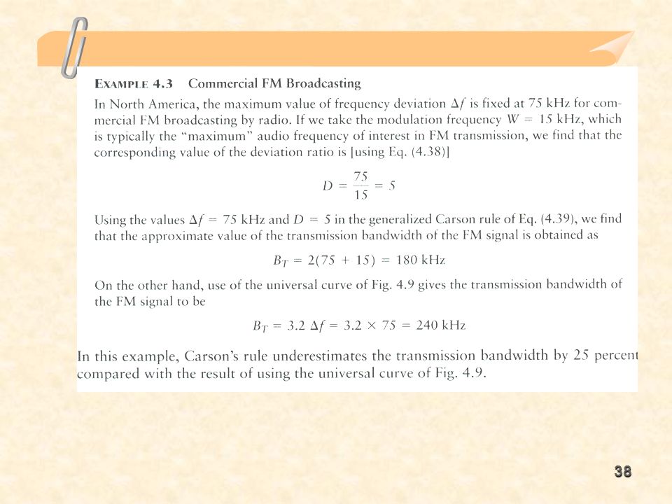
37. Arbitrary Modulating Wave
The bandwidth required to transmit an FM wave generated by an arbitrary modulating wave is based on a worst-case tone-modulation analysis
The deviation ratio D
The generalized Carson rule is
Fig. 4.9

39. 4.7 Generation of FM Waves Direct Method
A sinusoidal oscillator, with one of the reactive elements in the tank circuit of the oscillator being directly controllable by the message signal
The tendency for the carrier frequency to drift, which is usually unacceptable for commercial radio applications.
To overcome this limitation, frequency stabilization of the FM generator is required, which is realized through the use of feed-back around the oscillator
Indirect Method : Armstrong Modulator
The message signal is first used to produce a narrow-band FM, which is followed by frequency multiplication to increase the frequency deviation to the desired level.
Armstrong wide-band frequency modulator
The carrier-frequency stability problem is alleviated by using a highly stable oscillator
Fig. 4.10

40. Back
Next
Fig.4.10

41. A Frequency multiplier
A memoryless nonlinear device
The input-output relation of such a device is
A new FM wave is
Fig. 4.11

42. Back
Next
Fig.4.11

43. 4.8 Demodulation of FM Signals
Frequency Discriminator
The FM signal is
We can motivate the formulation of a receiver for doing this recovery by nothing that if we take the derivative of Eq. (4.44) with respect to time
A typical transfer characteristic that satisfies this requirement is

44. The complex envelope of the FM signal s(t) is
The slope circuit
The circuit is also not required to have zero response outside the transmission bandwidth
The complex envelope of the FM signal s(t) is
Fig. 4.12

45. Back
Next
Fig.4.12

46. Multiplication of the Fourier transform by j2πf is equivalent to differentiating the inverse Fourier transform
Application of the linearity property to the nonzero part of yields
the actual response of the slope circuit due to the FM wave s(t) is given by

47. Fig. 4.13 The envelope detector
Under ideal conditions, the output of the envelope detector is
The overall output that is bias-free
Fig. 4.13

48. Back
Next
Fig.4.13

49. Phase-Locked Loop
A feedback system whose operation is closely linked to frequency modulation
Three major components
Voltage-controlled oscillator (VCO)
Multiplier
Loop filter of a low-pass kind
Fig. 4.14, a closed-loop feedback system
VCO has bee adjusted so that when the control signal is zero, two conditions are satisfied
The frequency of the VCO is set precisely at the unmodulated carrier frequency fc of the incoming FM wave s(t)
The VCO output has a 90◦-degree phase-shift with respect to the unmodulated carrier wave.
Fig. 4.14

50. Back
Next
Fig.4.14

51. Suppose the incoming FM wave is
The FM wave produced by the VCO as
The multiplication of the incoming FM wave by the locally generated FM wave produces two components
A high-frequency component
A low-frequency component

52. Discard the double-frequency term, we may reduce the signal applied to the loop filter to
The phase error is
Eq. (4.62), (4.63), (4.65), and (4.60)constitute a linearized feedback model of the phase-locked loop
Loop-gain parameter of the phase lock loop

53. When the open-loop transfer function of a linear feedback system has a large magnitude compared with unity for all frequencies, the closed-loop transfer function of the system is effectively determined by the inverse of the transfer function of the feedback path.
The inverse of this feedback path is described in the time domain by the scaled differentiator
The closed-loop time-domain behavior of the phase-locked loop is described by the overall output v(t) produced in response to the angle Φ1(t) in the incoming FM wave s(t)
The magnitude of the open-loop transfer function of the phase-locked loop is controlled by the loop-gain parameter K0

54. We may relate the overall output v(t) to the input angle Φ1(t) by
Fig. 4.15

55. Back
Next
Fig.4.15

56. 4.9 Theme Example : FM Stereo Multiplexing
The specification of standards for FM stereo transmission is influenced by two factors
The transmission has to operate within the allocated FM broadcast channels
It has to be compatible with monophonic radio receivers
The multiplied signal is recovered by frequency demodulating the incoming FM wave
Fig. 4.16

57. Back
Next
Fig.4.16

58. 4.10 Summary and Discussion
Two kinds of angle modulation
Phase modulation (PM), where the instantaneous phase of the sinusoidal carrier wave is varied linearly with the message signal
Frequency modulation (FM), where the instantaneous frequency of the sinusoidal carrier wave is varied linearly with the message signal
Frequency modulation is typified by the equation
FM is a nonlinear modulation process
In FM, the carrier amplitude and therefore the transmitted average power is constant
Frequency modulation provides a practical method for the tradeoff of channel bandwidth for improved noise performance.

59. Back
Next
Fig.4.17
Fig. 4.17

60. Back
Next
Fig.4.18
Fig. 4.18

61. Back
Next
Fig.4.19
Fig. 4.19

62. Back
Next
Fig.4.20
Fig. 4.20

63. Back
Next
Fig.4.21
Fig. 4.21