1. Mad Money and Smart Money: The Discrepancy of Rationality between Options and Equity Markets Presented By Carl R. Chen – University of Dayton

2. I. Introduction We examine the impact of analyst’s recommendations on stocks and options Different reactions to the recommendations could distinguish trader types in these two markets We focus on the recommendations made by the popular CNBC Mad Money show hosted by Jim Cramer

3. The show is aired every weekday @ 6:00 p.m. The show draws more than 398,000 viewers daily Is this guy sexy?

4. Price Pressure vs. New Information Price Pressure Hypothesis Price could temporarily diverge from true value due to uninformed shift in excess demand New Information Hypothesis Price adjusts to new information permanently Test both the stock and options markets response to the Cramer’s stock recommendations Market that shows the price pressure effect is driven by the uninformed

5. II. Literature Stock Market Engelberg et al. (2007) and Balcarcel & Chen (2007) Motivation of Balcarcel & Chen Mad Money show produces a short-lived price pressure effect on the stock market  uninformed trading Options Market? No work related to the Mad Money effect there are literature related to the price discovery function of the options market

6. Options price does not predict stock (spot) price Stock Options: Stephan & Whaley (1990), Chan et al (1993), O’Connor et al (1999), Chan et al (2002) Currency Options: Brenner et al (1996), Pan et al (1996) Informed trades occur in the options market Using Hasbrouck’s (1995) information share analysis, Chakravarty, Gulen, Mahyhew (2004) find that 17% of the price discovery occurs in the options market Easley, O’Hara, Srinivas (1998), Pan, Poteshman (2003) use signed options volume to show that options markets contain information of the underlying asset price changes Cao et al (2000): abnormal trading before takeover announcements

7. III. Data and Methodology  Data Final sample contains 368 buy and 358 sell recommendations for the months of August and September 2005 Daily stock returns are taken from CRSP Stock dividend yields are from COMPUSTAT Daily options data are obtained from the Market Data Express (MDX) by CBOE To minimize the non-synchronous trading, we match MDX underlying stock price with intraday bid-ask from Trade and Quote (TAQ) We drop the observation when stock price in options data differs from CRSP by more than 0.5%

8. Methodology A.Event Study Procedure R it =α i + β i R mt + ε it, t=-124,…, -5 AR it = R it – (α` i + β` i R mt ) = ε` it, t = 1, 2,…, 30

9. We also compute the average abnormal share turnover (ATO) and average abnormal bid-ask spread (ASPREAD) for each day follow the same procedure In the revised version of the paper (in progress) We use three-factor model to compute the abnormal returns We expand the sample to cover more than 1,000 recommendations

10. B. Implied Price Changes in the Options Market 1. The Sequential Approach  Since  Implied volatility of the previous period serves as a proxy of  t. Together with options premium O t and R t, we estimate the implied stock price backwardly using the Generalized Newton Method algorithm (see Chakravarty et al 2004). This is a direct measurement of the stock price embedded in options Where R t represents other observable variables such as risk- free rate, options maturity, and strike price, then

11. 2. The Option Boundary Approach This approach gauges the degree of divergence between option-implied and actual stock price American option boundary with market friction of Bodurtha and Courtadon (1986) is employed This is a model-free estimate, but not a direct measure of stock price With market frictions, the upper boundaries for American call and put are as follows:  (P a + S a – Xe -rt ) + (T X +T S +T P )≥ C b - T c  (C a - S b e -qt + X) + (T X +T S +T C )≥ P b -T p

12. S, P, C, X, r, q and t are stock price, put premium, call premium, strike price, risk-free rate, dividend yield, and time to maturity. Superscript « a » and « b » denore ask and bid of the quotes. T represents transaction cost for trading respective instruments. S a ≥ C b – P a +Xe -rxt – (T x +T s +T p +T c ) =L S b ≤ [C a – P b +X + (T x +T s +T p +T c )]/e -qt =H (L – S a )  distance between lower bound and the observed stock price (S b – H)e –qt  distance between higher bound and observed stock price

13.  Divergence= (C a + C b - P a – P b ) - (S a + S b e -qt ) + X(1+e -rt )  A positive (negative) “Divergency” indicates that the implied stock price is more likely to be larger (smaller) than the observed stock price. |-----------------------  --------------*---------*-----------  ---------------------------------| Low Sb Sa High |_______Divergence=0_______| Low High |________Divergence<0_______| Low  High  |_________ Divergence>0________|

14. 3. Options data  Three options maturities:  short: 10-30 days;  Mid: 31-60 days;  Long: 61-120 days  Three options moneyness  OTM:  =0.02~0.45;  ATM:  =0.45~0.55;  ITM:  =0.55~0.98

15. IV. Empirical Results Table 1: Summary Statistics

16. Table 2: Summary Statistics of the Options Data Panel A – Call Options for the Buy Recommendations

17. Table 2: Panel B – Call Options for Sell Recommendations

18. Table 2: Panel C – Put Options for Buy Recommendations

19. Table 2: Panel D – Put Options for Sell Recommendations

20. Table 3: The Price Pressure Effect (Stock Markets)

22. Table 4: The Price Pressure Effect (Options Markets) Panel A – Buy Recommendations Only Days 1 is reported Synthetic Short stock

23. Table 4: The Price Pressure Effect (Options Markets) Panel B – Sell Recommendations

24. Table 5: Correlations between Abnormal Stock Returns and Abnormal Implied Price Changes (day -124 ~ -5)

25. Table 6: Effect on Options Trading Panel A – Buy Recommendations

26. Table 6: Effect on Options Trading Panel B – Sell Recommendations

27. Table 7: Trading Profit (Long Short-term Puts) R t = (V t – O t )/O t Day -125 ~ -30 Buy a day after recommendation Modified Johnson t- test  In the revised version where longer data period is employed, we find most of the profit opportunity disappeared in the latter period. Get rich quick?

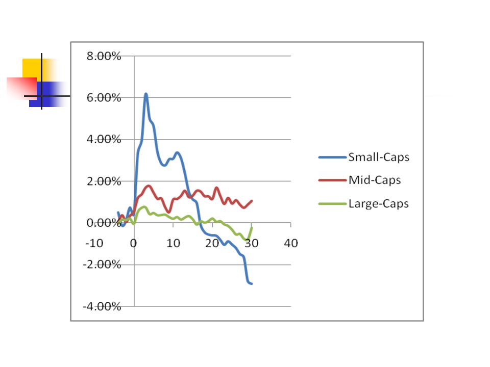
28. V. Conclusions Small-cap stocks show a short-lived price run-up followed by a price reversal for the stocks Cramer recommended to buy  evidence of uninformed trading Options markets largely lack such price pressure effect  informed trading Short-term ITM put options react counter the buy recommendations. Bid-ask spreads decreased and trading increased  Take advantage of naïve trading in the spot markets. Buy short-term puts generate high profits during the event periods. ITM puts generate the highest returns. Longer data period and different market model are employed in the revision. Results are not materially changed. There is evidence that market learns.