1. ENERGY UPDATE! Today’s Material Climate Forcing Climate Forcing Project Discussions Project Discussions Week 10: Impact of Fossil Fuels (ch 6) Week 10: Impact of Fossil Fuels (ch 6) Week 11: Hydro, Wind, Biomass (ch 10) Week 11: Hydro, Wind, Biomass (ch 10) Week 12: Vet’s Day, Mid Term II Preview 11/12/14 Week 12: Vet’s Day, Mid Term II Preview 11/12/14 Week 13: Is Earth Warming (ch 14), Mid Term II 11/19/14 (notebooks due) Week 13: Is Earth Warming (ch 14), Mid Term II 11/19/14 (notebooks due) Week 14: Presentations Week 14: Presentations Week 15: Presentations Week 15: Presentations

2. Renewables cutting US emissions more than gas as coal consumption drops http://www.greenpeace.org.uk/newsdesk/energy/data/data-what-accounts-huge-cut-us-coal-use-2007 License: All rights reserved. Credit: Greenpeace Wind power, not shale gas, is the biggest single cause of the fall in US emissions from coal use, according a new analysis of US data by Energydesk. The fall in US coal consumption since 2007 is to a larger extent down to improved energy efficiency and an increase in renewable generation than to use of shale gas, Greenpeace analyst Lauri Myllvirta has found. Between 2007-13 the US experienced the largest fall in coal usage ever experienced by any country, with renewables, energy efficiency and shale gas together picking up the slack. The switch from coal has led to lower emissions from the power sector, which has largely been attributed to fracking.

3. 21% fall in coal Between 2007 and 2013 US coal-fired generation fell by 21%, leaving a vacuum of 43 terawatt-hours to be filled by other types of energy, equivalent to more than the power consumption of the entire U.S. West Coast. What is the impact on emissions? Here’s where the rise of renewables and energy efficiency gets even more pronounced.

4. Where’s this headed? US coal consumption will further fall by up to 25% by 2020, according to a report from Wall Street analysts.

5. Negative feedback associated with clouds. An initial increase in Earth’s temperature results in increased evaporation and therefore more clouds. Because clouds are highly reflective, they increase the planet’s albedo. More reflected sunlight means less solar energy is absorbed by the Earth system. The final effect, therefore, is to moderate the initial temperature increase. This is only one of many cloud feedbacks. The feedback works in both directions, so the same diagram applies if the increases and decreases are interchanged.

6. Ice–albedo feedback is a positive feedback effect. A temperature increase results in melting sea ice, exposing dark seawater. Earth’s albedo is reduced, resulting in more solar energy absorption. This, in turn, exacerbates the initial temperature increase. Ice–albedo feedback would also exacerbate an initial cooling.

7. Changes in climate forcings since 1750. Positive forcings result in warming; negative forcings result in cooling. Error bars show uncertainties, some of which are relatively large. The well-mixed greenhouse gases are stacked in a single bar. The only natural forcing shown here is solar forcing, resulting from changes in the Sun’s power output. Not shown are anthropogenic forcings due to aviation- induced clouds (contrails) and the sporadic natural forcing associated with individual volcanic eruptions. This graph, based on 2007 IPCC data, may underestimate the positive forcing due to black carbon aerosol.

8. Methane is 26 times more effective at infrared absorption than is a molecule of CO 2. However, Methane has a much shorter atmospheric lifetime.

9. Major sources of global anthropogenic CO 2 emissions in the early twenty-first century. Four-fifths of the CO 2 comes from fossil fuel combustion. The CO 2 emissions from land-use changes are largely from deforestation in the tropics. All of these emissions total about 10 Gt of carbon annually.

10. Atmospheric CO 2, CH 4, and N 2 O concentration history over the industrial era (right) and from year 0 to the year 1750 (left), determined from air enclosed in ice cores and firn air (color symbols) and from direct atmospheric measurements (blue lines, measurements from the Cape Grim observatory)

11. http://cliffmass.blogspot.com/2013/10/ocean-acidification-and-northwest.html The figure above shows the increase in atmospheric CO2 (red line), the increase in CO2 gas of the waters in the middle of the Pacific (dark blue), and the decline of ph from 8.11 to 8.07 since 1988 (24 years, light blue). How do we know the CO 2 rise is due to anthropogenic emissions? 1.We know how much fossil fuels we burn. 2.CO 2 concentration is higher in northern Hemisphere, where we burn more of it. 3. 14 C: 12 C ratio is decreasing, as expected if atmosphere is flooded with old carbon (no 14 C in fossil fuels).

12. http://earthobservatory.nasa.gov/blogs/climateqa/mauna-loa-co2-record/

13. Launch land connection video Watching the Earth Breathe: An Animation of Seasonal Vegetation and its effect on Earth's Global Atmospheric Carbon Dioxide http://svs.gsfc.nasa.gov/vis/a000000/a003900/a003947/index.html

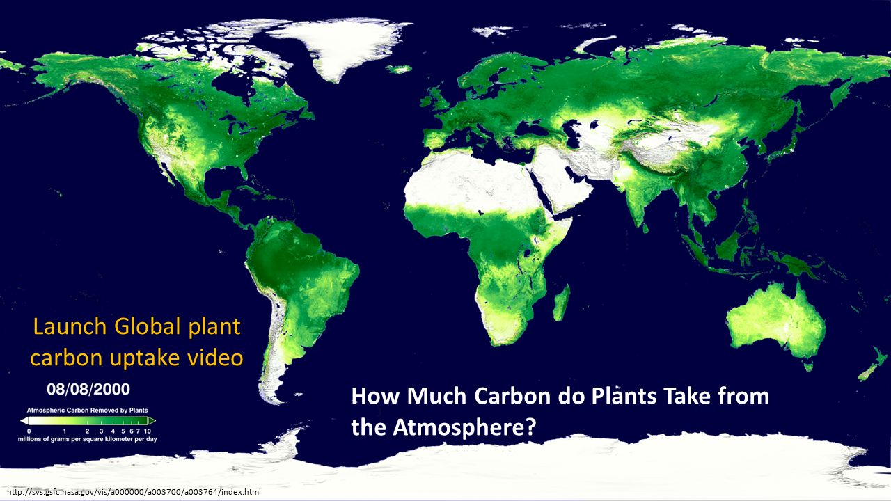
14. Launch Global plant carbon uptake video How Much Carbon do Plants Take from the Atmosphere? http://svs.gsfc.nasa.gov/vis/a000000/a003700/a003764/index.html

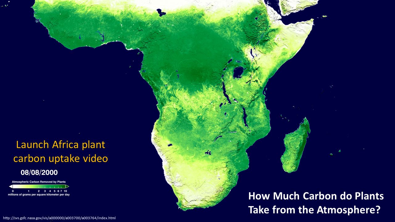
15. Launch Africa plant carbon uptake video How Much Carbon do Plants Take from the Atmosphere? http://svs.gsfc.nasa.gov/vis/a000000/a003700/a003764/index.html

16. The carbon cycle. Carbon reservoirs are in gigatonnes (Gt) of carbon; flows (arrows) are in gigatonnes per year. All numbers are approximate and have been rounded to integers. Fossil fuel combustion and deforestation are the dominant anthropogenic factors upsetting the carbon cycle. Today, carbon is accumulating in the atmosphere at about 4 Gt per year. What are the imbalances? Why might these imbalances not be guaranteed into the future?

17. Simplified schematic of the global carbon cycle. Numbers represent reservoir mass, also called ‘carbon stocks’ in Pg C (1 Pg C = 10 15 g C) and annual carbon exchange fluxes (in Pg C yr–1). Black numbers and arrows indicate pre-industrial reservoir mass and exchange fluxes. Black numbers and arrows indicate pre-industrial reservoir mass and exchange fluxes. Red arrows and numbers indicate annual ‘anthropogenic’ fluxes averaged over the 2000– 2009 time period. Red arrows and numbers indicate annual ‘anthropogenic’ fluxes averaged over the 2000– 2009 time period.

18. http://earthobservatory.nasa.gov/Features/OceanCarbon/ In the short term, the ocean absorbs atmospheric carbon dioxide into the mixed layer, a thin layer of water with nearly uniform temperature, salinity, and dissolved gases. Wind- driven turbulence maintains the mixed layer by stirring the water near the ocean’s surface. Over the long term, carbon dioxide slowly enters the deep ocean at the bottom of the mixed layer as well in in regions near the poles where cold, salty water sinks to the ocean depths.

19. CO 2 dissolves in water to form carbonic acid, H 2 CO 3. (It is worth noting that carbonic acid is what eats out limestone caves from our mountains.) In the oceans, carbonic acid releases hydrogen ions (H+), reducing pH, and bicarbonate ions (HCO 3 -). CO 2 + H 2 O  H 2 CO 3 => H + + HCO 3 - (1) The additional hydrogen ions released by carbonic acid bind to carbonate ions (CO 3 2- ), forming additional bicarbonate ions, HCO 3 -. H + + CO 3 2- => HCO 3 - (2) This reduces the concentration of CO 3 2-, making it harder for marine creatures to take up CO 3 2- to form the calcium carbonate needed to build their exoskeletons. Ca 2+ + CO 3 2- => CaCO 3 (3) The two main forms of calcium carbonate used by marine creatures are calcite and aragonite. Decreasing the amount of carbonate ions in the water makes conditions more difficult for both calcite users (phytoplankton, foraminifera and coccolithophore algae), and aragonite users (corals, shellfish, pteropods and heteropods).

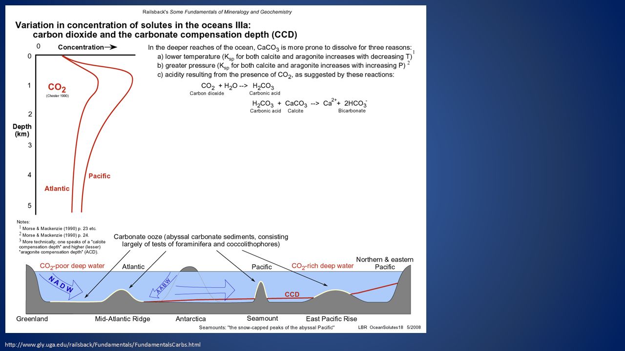
20. http://www.gly.uga.edu/railsback/Fundamentals/FundamentalsCarbs.html

21. http://earthobservatory.nasa.gov/Features/OceanCarbon/ The concentration of carbon dioxide (CO 2 ) in ocean water (y axis) depends on the amount of CO 2 in the atmosphere (shaded curves) and the temperature of the water (x axis). This simplified graph shows that as atmospheric CO 2 increases from pre- industrial levels (blue) to double (2X) the pre-industrial amounts (light green), the ocean CO 2 concentration increases as well. However, as water temperature increases, its ability dissolve CO 2 decreases. Global warming is expected to reduce the ocean’s ability to absorb CO 2, leaving more in the atmosphere…which will lead to even higher temperatures.

22. In certain areas near the polar oceans, the colder surface water also gets saltier due to evaporation or sea ice formation. In these regions, the surface water becomes dense enough to sink to the ocean depths. This pumping of surface water into the deep ocean forces the deep water to move horizontally until it can find an area on the world where it can rise back to the surface and close the current loop The oceans are mostly composed of warm salty water near the surface over cold, less salty water in the ocean depths.

23. http://svs.gsfc.nasa.gov/vis/a000000/a003600/a003658/ Launch thermohaline conveyor video

24. http://svs.gsfc.nasa.gov/vis/a000000/a004100/a004110/ Launch RCP 2.6 video These visualizations represent the mean output of how certain groups of CMIP5 models responded to four different scenarios defined by the IPCC called Representative Concentration Pathways (RCPs). These four RCPs - 2.6, 4.5, 6 and 8.5 - represent a wide range of potential worldwide greenhouse gas emissions and sequestration scenarios for the coming century. The pathways are numbered based on the expected Watts per square meter - essentially a measure of how much heat energy is being trapped by the climate system - each scenario would produce

25. http://svs.gsfc.nasa.gov/vis/a000000/a004100/a004110/ Launch RCP 8.5 video The carbon dioxide concentrations in the year 2100 for each RCP are: RCP 2.6: 421 ppm RCP 4.5: 538 ppm RCP 6: 670 ppm RCP 8.5: 936 ppm