1. CG Algorithms and Implementation: “From Vertices to Fragments” Angel: Chapter 6 OpenGL Programming and Reference Guides, other sources. ppt from Angel, AW, van Dam, etc. CSCI 6360/4360

2. Introduction Implementation -- Algorithms Angel’s chapter title: “From Vertices to Fragments” –… and in the chapter are “various” algorithms From one perspective of pipeline: Next steps in viewing pipeline: –Clipping Eliminating objects that lie outside view volume - and, so, not visible in image –Rasterization Produces fragments from remaining objects –Hidden surface removal (visible surface determination) Determines which object fragments are visible

3. Introduction Implementation -- Algorithms Need to consider another perspective, as well Next steps in viewing pipeline: –Clipping –Rasterization Produces fragments from remaining objects –Hidden surface removal (visible surface determination) Determines which object fragments are visible Show objects (surfaces)not blocked by objects closer to camera And next week …

4. Introduction Implementation -- Algorithms Next steps in viewing pipeline: –Clipping –Rasterization –Hidden surface removal (visible surface determination) Will consider above in some detail in order to give feel for computational cost of these elements “in some detail” = algorithms for implementing –… algorithms that are efficient –Same algorithms for any standard API –Will see different algorithms for same basic tasks

5. About Implementation Strategies Angel: At most abstract level … –Start with application program generated vertices –Do stuff like transformation, clipping, … –End up with pixels in a frame buffer Can consider two basic strategies Will see again in hidden surface removal Object-oriented -- An object at a time … –For each object Render the object –Each object has series of steps Image-oriented -- A pixel at a time … –For each pixel Assign a frame buffer value –Such scanline based algorithms exploit fact that in images values from one pixel to another often don’t change much Coherence –So, can use value of a pixel in calculating value of next pixel Incremental algorithm

6. Tasks to Render a Geometric Entity 1 Review and Angel Explication Angel introduces more general terms and ideas, than just for OpenGL pipeline… –Recall, chapter title “From Vertices to Fragments” … and even pixels –From definition in user program to (possible) display on output device –Modeling, geometry processing, rasterization, fragment processing Modeling –Performed by application program, e.g., create sphere polygons (vertices) –Angel example of spheres and creating data structure for OpenGL use –Product is vertices (and their connections) –Application might even reduce “load”, e.g., no back-facing polygons

7. Tasks to Render a Geometric Entity 2 Review and Angel Explication Geometry Processing –Works with vertices –Determine which geometric objects appear on display –1. Perform clipping to view volume Changes object coordinates to eye coordinates Transforms vertices to normalized view volume using projection transformation –2. Primitive assembly Clipping object (and it’s surfaces) can result in new surfaces (e.g., shorter line, polygon of different shape) Working with these “new” elements to “re-form” (clipped) objects is primitive assembly Necessary for, e.g., shading –3. Assignment of color to vertex Modeling and geometry processing called “front-end processing” –All involve 3-d calculations and require floating-point arithmetic

8. Tasks to Render a Geometric Entity 3 Review and Angel Explication Rasterization –Only x, y values needed for (2-d) frame buffer … as the frame buffer is what is displayed –Rasterization, or scan conversion, determines which fragments displayed (put in frame buffer) For polygons, rasterization determines which pixels lie inside 2-d polygon determined by projected vertices –Colors Most simply, fragments (and their pixels) are determined by interpolation of vertex shades & put in frame buffer –Output of rasterizer is in units of the display (window coordinates)

9. Tasks to Render a Geometric Entity 4 Review and Angel Explication Fragment Processing –Colors OpenGL can merge color (and lighting) results of rasterization stage with geometric pipeline E.g., shaded, texture mapped polygon (next chapter) –Lighting/shading values of vertex merged with texture map For translucence, must allow light to pass through fragment Blending of colors uses combination of fragment colors, using colors already in frame buffer –e.g., multiple translucent objects –Hidden surface removal performed fragment by fragment using depth information –Anti-aliasing also dealt with

10. Efficiency and Algorithms For cg illumination/shading, saw how role of efficiency drove algorithms –Phong shading is “good enough” to be perceived as “close enough” to real world –Close attention to algorithmic efficiency Similarly, for often calculated geometric processing efficiency is a prime consideration Will consider efficient algorithms for: –Clipping –Line drawing –Visible surface drawing

11. Recall, Clipping … Scene's objects are clipped against clip space bounding box –Eliminates objects (and pieces of objects) not visible in image –Efficient clipping algorithms for homogeneous clip space Perspective division divides all by homogeneous coordinates, w Clip space becomes Normalized Device Coordinate (NDC) space after perspective division

12. Clipping Efficiency matters

13. Clipping is performed many times in cg pipeline –Depending on algorithms, number of lines, polygons Different kinds of clipping –2D against clipping window, 3D against clipping vol. Easy for line segments of polygons –Polygons can be handled in other ways, too E.g., Bounding boxes Hard for curves and text –Convert to lines and polygons first Will see, 1st example of a cg algorithm –Designed for very efficient execution –Efficiency includes: multiplication vs. addition use of Boolean vs. arithmetic operations Integer vs. real Space complexity Even the “constant” in time complexities

14. Clipping - 2D Line Segments Could clip using brute force –Compute intersections with all sides of clipping window Computing intersections is expensive –To explicitly find intersection, essentially solve y = mx + b Use lines end points to find slope and intercept See if line is in there –Requires multiplication/division

15. Cohen-Sutherland Algorithm An example clipping algorithm Cohen-Sutherland clipping algorithm considers all different cases for where line may be wrt clipping region E.g., will first eliminate as many cases as possible without computing intersections –E.g., both ends of line outside (line C-D), or inside (line A-B) –Again, computing intersections is expensive Start with four lines that determine sides of clipping window –As if extending sides, top, and bottom of window out –Will use x min, x max, y min,y max, in algorithm x = x max x = x min y = y max y = y min

16. Consider Cases: Where Endpoints Are Based on relationship of endpoints and clipping region x min, x max, y min, y max, will define cases Case 1: –Both endpoints of line segment inside all four lines –Draw (accept) line segment as is Case 2: –Both endpoints outside all lines and on same side of a line –Discard (reject) the line segment –“trivially reject” Case 3: –One endpoint inside, one outside –Must do at least one intersection Case 4: –Both endpoints outside, not on same side –May have part inside –Must do at least one intersection x= x min y = y max y = y min x = x max x = x min y = y max y = y min

17. Defining Outcodes A representation for efficiency For each line endpoint defines an outcode: –Endpoint includes both x 1, y 1 and x 2, y 2 –4 bits for each endpoint: b 0 b 1 b 2 b 3, b 0 = 1 if y > y max, 0 otherwise b 1 = 1 if y < y min, 0 otherwise b 2 = 1 if x > x max, 0 otherwise b 3 = 1 if x < x min, 0 otherwise Examples in red with blue ends at right: –Tedious, but automatic –E.g., left line outcodes: 0000, 0000 –E.g., right line outcodes: 0110, 0010 Outcodes divide space into 9 regions Computation of outcode requires at most 4 subtractions –E.g., y 1 - y max Testing of outcodes can be done with bitwise comparisons x= x min y = y max y = y min

18. Now will consider each case using outcodes … Based on relationship of endpoints and clipping region x min, x max, y min, y max, will define cases Case 1: –Both endpoints of line segment inside all four lines –Draw (accept) line segment as is Case 2: –Both endpoints outside all lines and on same side of a line –Discard (reject) the line segment –“trivially reject” Case 3: –One endpoint inside, one outside –Must do at least one intersection Case 4: –Both endpoints outside, not on same side –May have part inside –Must do at least one intersection x= x min y = y max y = y min x = x max x = x min y = y max y = y min

19. Using Outcodes, Case 1 Example from Angel Based on relationship of endpoints and clipping region x min, x max, y min, y max, will define cases Case 1: –Both endpoints of line segment inside all four lines –Draw (accept) line segment as is AB: outcode(A) = outcode(B) = 0 –A = 0000, B = 0000 –Accept line segment x= x min y = y max y = y min

20. Using Outcodes, Case 2 Example from Angel Case 2: –Both endpoints outside all lines and on same side of a line –Discard (reject) the line segment –“trivially reject EF: outcode(E) && outcode(F)  0 –&& is bitwise logical AND –E = 0010, F = 0010 –Both outcodes have 1 bit in same place –Line segment is outside of corresponding side of clipping window –Reject – typically, most frequent case x= x min y = y max y = y min

21. Using Outcodes, Case 3 Example from Angel Case 3: –One endpoint inside, one outside –Must do at least one intersection CD: outcode (C) = 0, outcode(D)  0 –C = 0000, D = anything else –Here, D = 0010 –Do need to compute intersection –Location of 1 in outcode (D) determines which edge to intersect with –So, “shortened” line is what is displayed C – D’ –Note: If there were a segment from A to a point in a region with 2 ones in outcode, might have to do two intersections D’ x = x max x = x min y = y max y = y min

22. Using Outcodes, Case 4 Example from Angel Case 4: –Both endpoints outside, not on same side –May have part inside –Must do at least one intersection GH, IJ (same outcodes), neither zero, but && of endpoints = zero –G (and I) = 0001, H (and J) = 1000 –Test for intersection –If found, shorten line segment by intersecting with one of sides of window –Compute outcode of intersection (new endpoint of shortened line segment) –(Recursively) reexecute algorithm I’ J’ x = x max x = x min y = y max y = y min

23. Efficiency and Extension to 3D Very efficient in many applications –Clipping window small relative to size of entire data base –Most line segments are outside one or more side of the window and can be eliminated based on their outcodes Inefficient, when code has to be reexecuted for line segments that must be shortened in more than one step For 3 dimensions –Use 6-bit outcodes –When needed, clip line segment against planes

24. Rasterization

25. End of geometry pipeline (processing) – –Putting values in the frame buffer (or raster) –As, write_pixel (x, y, color) At this stage, fragments – clipped, colored, etc. at level of vertices, are turned into values to be displayed –(deferring for a moment the question of hidden surfaces and colors) Essential question is “how to go from vertices to display elements?” –E.g., lines Algorithmic efficiency is a continuing theme

26. Drawing Algorithms As noted, implemented in graphics processor –Used bazillions of times per second –Line, curve, … algorithms Line is paradigm example –most common 2D primitive - done 100s or 1000s or 10s of 1000s of times each frame –even 3D wireframes are eventually 2D lines –optimized algorithms contain numerous tricks/techniques that help in designing more advanced algorithms Will develop a series of strategies, towards efficiency

27. Drawing Lines: Overview Recall, fundamental “challenge” of computer graphics: –Representing the analog (physical) world on a discrete (digital) device –Consider a very low resolution display: Sampling a continuous line on a discrete grid introduces sampling errors: the “jaggies” –For horizontal, vertical and diagonal lines all pixels lie on the ideal line: special case For lines at arbitrary angle, pick pixels closest to the ideal line Will consider several approaches –But, “fast” will be best

28. Strategy 1 ­ Really Basic Algorithm First, the (really) basic algorithm: –Find equation of line that connects 2 pts, P x,y, Q x,y –y = mx + b –m =  y /  x, where  x = x end – x start,  y = y end – y start Starting with the leftmost point P, –increment x by 1 and calculate y = mx + b at each x point/value –where m = slope, b = y intercept for x = P x to Q x y = round (m * x + b)// compute y write-pixel (x, y) This works, but uses computationally expensive operations (multiply) at each step –Perhaps worked for your homework –And do note that when turn on a pixel, in fact does approximate an ideal line P x,y Q x,y

29. Strategy 2 ­ Incremental Algorithm, 1 So, (really) basic algorithm: for x = P x to Q x y = round (m * x + b)// compute y write-pixel (x, y) Can modify basic algorithm to be an incremental algorithm –Use current state of computation in finding next state i.e., incrementally going toward the solution –Not “recompute” the entire solution, as above – Not same computation regardless of where are Use partial solution, here, last y value, to find next value Modify (really) Basic Algorithm to just add slope, vs. multiply – next slide m =  y /  x// compute slope (to be added) y = m * P x + b// still multiply to get first y value for x = P x, Q x write-pixel (x, round(y)) y = y + m // increment y for next value, just by adding Make incremental calcs based on preceding step to find next y value –Works here because going unit/1 to right, incrementing x by 1 and y by (slope) m P x,y Q x,y

30. Strategy 2 ­ Incremental Algorithm, 2 Incremental algorithm m =  y /  x// slope y = m * P x + b// first y value for x = P x to Q x write-pixel (x, round(y)) y = y + m // inc y for next Definite improvement over basic algorithm Still problems –Still too slow a.Rounding integers takes time b.Variables y and m must be a real or fractional binary because slope is a fraction Ideally, want just integers and add m

31. Strategy 3 ­ Midpoint Line Algorithm Midpoint line algorithm (MLA) considers that “ideal” line is in fact approximated on a raster (pixel based) display Hence, will be “error” in where ideal line should be and how it is represented by turning on pixels Will use amount of “possible error” to decide which pixel to turn on for successive steps … and will do this by only adding and comparing (=, >, <) error

32. Strategy 3 ­ MLA, 1 Assume that the (ideal) line's slope is shallow and positive (0 < m < 1). –Other slopes can be handled by suitable reflections about principal axes Note are calculating “ideal line” and turning on pixels as approximation Assume that we have just selected the pixel P at (x p,y p ) Next, must choose between: –pixel to right (pixel E), or –pixel one right and one up (pixel NE) Let Q be intersection point of line being scan­converted with grid line at x = x p + 1 Note that pixel turned on is not exactly on ideal line – so, “error” Q

33. Strategy 3 - MLA, 2 Observe on which side of (ideal) line the midpoint M lies: –E pixel closer to line if midpoint lies above line –NE pixel closer to line if midpoint lies below line (Ideal) line passes between E and NE –Point closer to point Q must be chosen Either E or NE Error: (here, ) –Vertical distance between chosen pixel and actual line - always <= ½ Here, algorithm chooses NE as next pixel for line shown Now, find a way to calculate on which side of line midpoint lies

34. MLA – Use Equation of Line for Selection How to choose which pixel, based on M and distance of M from ideal line Line equation as a function, f(x): –y = m * x + b –y = dy/dx * x + b And line equation as an implicit function: –f(x, y) = a*x + b*y + c = 0 –From above, algebraically (multiply by dx) y * dx = dy * x + b * dx –So, algebraically, a = dy, b = ­dx, c = b*dx, a>0 for y 0 <y 1 Properties (proof by case analysis): –f(x m, y m ) = 0 when any point M is on line –f(x m, y m ) < 0 when any point M above line –f(x m, y m ) > 0 any point M below line - here Decision (to choose E or NE) will be based on value of function at midpoint –M at (x p+1, y p+1/2 ) – ½ - midpoint

35. MLA, Decision Variable So, find a way to (efficiently) calculate on which side of line midpoint lies And that’s what we just saw –E.g., f(x m, y m ) < 0 when any point M above line Decision variable d: –Only need sign (fast) of f (x p+1, y p+1/2 ) to see where the line lies, –and then pick nearest pixel. –d = f (x p+1, y p+1/2 ) if d > 0 choose pixel NE. if d < 0 choose pixel E. if d = 0 choose either one consistently. Next, how to update d: –On basis of picking E or NE, figure out the location of M to that pixel, and the corresponding value of d for the next grid line

36. How to update d, if E was chosen: M is incremented by one step in x direction Recall, f(x, y) = a*x + b*y + c = 0 and rewrite –To get the incremental difference, DE, subtract d old from d new d new = f(x p + 2, y p + 1/2 ) = a(x p +2 ) + b(y p + 1/2 ) + c d old = a(x p + 1 ) + b(y p + 1/2 ) + c Derive value of decision variable at next step incrementally without computing f(M) directly (recall “incremental algorithm): –d new = d old + DE = d old + dy –DE = a = dy DE can be thought of as the correction, or update factor, to take d old to d new –(and this is the insight: “carrying along the error, vs. recalculating”). –d new = d old + a Called “forward difference”

37. How to update d, ff NE was chosen: M is incremented by one step each in both the x and y directions –d new = f(x p+2, y p+3/2 ) –d new = a(x p+2 ) + b(y p+3/2 ) + c Subtract d old from d new to get the incremental difference –d new = d old + a + b –DNE = a + b = dy ­ dx So, incrementally, –d new = d old + DNE = d old + dy ­ dx

38. MLA Summary At each step, algorithm chooses between 2 pixels based on sign of decision variable, d, calculated in previous iteration Update decision variable, d, by adding either DE or DNE to old value d depending on choice of pixel. Note - First pixel is first endpoint (x 0, y 0 ), so can directly calc init val of d for choosing between E and NE. First midpoint is at (x 0 + 1, y 0 + 1/2) F(x 0+1, y 0+1/2 ) = a(x 0 + 1 ) + b(y 0 + 1/2 ) + c = ax 0 + by 0 + c + a + b/2 = F(x 0, y 0 ) + a + b/2 But (x 0, y 0 ) is point on line and F(x 0, y 0 ) = 0 Therefore, d start = a + b/2 = dy ­ dx/2. Use d start to choose the second pixel, etc. To eliminate fraction in d start: Redefine F by multiplying it by 2; F(x,y) = 2(ax + by + c). This multiplies each constant and the decision variable by 2, but does not change the sign.

39. Hidden Surface Removal Or, Visible Surface Determination (VSD)

40. Recall, Projection … Projectors View plane (or film plane) Direction of projection Center of projection –Eye, projection reference point

41. About Visible Surface Determination, 1 Have been considering models, and how to create images from models –e.g., when viewpoint/eye/COP changes, transform locations of vertices (polygon edges) of model to form image In fact, projectors are extended from front and back of all polygons –Though only concerned with “front” polygons Projectors from front (visible) surface only

42. About Visible Surface Determination, 2 To form image, must determine which objects in scene obscured by other objects –Occlusion Definition of visible surface determination (VSD): –Given a set of 3-D objects and a view specification (camera), determine which lines or surfaces of the object are visible –Also called Hidden Surface Removal (HSR)

43. Visible Surface Determination: Historical notes Problem first posed for wireframe rendering –doesn’t look too “real” (and in fact is ambiguous) Solution called “hidden-line (or surface) removal” –Lines themselves don’t hide lines Lines must be edges of opaque surfaces that hide other lines –Some techniques show hidden lines as dotted or dashed lines for more info Hidden surface removal appears as one stage

44. Classes of VSD Algorithms Different VSD algorithms have advantages and disadvantages: 0. “Conservative” visibility testing: –only trivial reject - does not give final answer E.g., back-face culling, canonical view volume clipping Have to feed results to algorithms mentioned below 1. Image precision –resolve visibility at discrete points in image Z-buffer, scan-line (both in hardware), ray-tracing 2. Object precision –resolve for all possible view directions from a given eye point

45. Image Precision Resolve visibility at discrete points in image Sample model, then resolve visibility –raytracing, Z-buffer, scan-line operate on display primitives. e.g., pixels, scan-lines visibility resolved to the precision of the display (very) High Level Algorithm: for (each pixel in image, i.e., from COP to model) { 1. determine object closest to viewer pierced by projector thru pixel 2. draw pixel in appropriate color } Complexity: –O( n. p), where n = objects, p = pixels, from above for loop or just, at each pixel consider all objects and find closest point

46. Object Precision, 1 Resolve for all possible view directions from a given eye point Each polygon is clipped by projections of all other polygons in front of it Irrespective of view direction or sampling density Resolve visibility exactly, then sample the results Invisible surfaces are eliminated and visible sub-polygons are created –e.g., variations on painter's algorithm, poly’s clipping poly’s, 3-D depth sort, BSP: binary- space partitions

47. Object Precision, 2 (very) High Level Algorithm for (each object in the world) { 1. determine parts of object whose view is unobstructed by other parts of it or any other object 2. draw pixel in appropriate color } Complexity: –O( n 2 ), where n = number of objects –from above for loop or just –must consider all objects (visibility) interacting with all others –(but, even when n << p, “steps” are longer, as a constant factor)

48. “Ray Casting” for VSD Recall ray tracing –For each pixel, follow the path of “light” back to the source, considering surface properties (smoothness, color) –“Color” of pixel is result For “ray casting”, –Just follow a ray from cop to first polygon encountered – and that polygon will be visible, and others won’t be –Conceptually simple, but not used An image precision algorithm –Time proportional to number of pixels

49. Painter’s Algorithm Another simple algorithm … –Way to resolve visibility –Create drawing order, each poly overwriting the previous ones guarantees correct visibility at any pixel resolution Strategy is to work back to front –Find a way to sort polygons by depth (z), then draw them in that order Sort of polygons by smallest (farthest) z-coordinate in each polygon Draw most distant polygon first, then work forward towards the viewpoint (“painters’ algorithm”) An object precision algorithm –Time proportional to number of objs/polys

50. Painter’s Algorithm Problems Intersecting polygons present a problem Even non-intersecting polygons can form a cycle with no valid visibility order:

51. Back-Face Culling Overview Back-face culling directly eliminates (culls) polygons not facing viewer Makes sense given constraint of convex (no “inward” face) polygons Computationally, can eliminate back faces by: –Line of sight calculations –Plane half-spaces In practice, –Surface (and vertex) normals often stored with vertex list representations –Normals used both in back face culling and illumination/shading models

52. Back-Face Culling Line of Sight Interpretation Line of Sight Interpretation Use outward normal (ON) of polygon to test for rejection LOS = Line of Sight, –The projector from the center of projection (COP) to any point P on the polygon. –(note: For parallel projections LOS = DOP = direction of projection) If normal is facing in same direction as LOS, it’s a back face: –Use cross-product – if LOS ON >= 0, then polygon is invisible—discard – if LOS ON < 0, then polygon may be visible

53. Back-Face Culling OpenGL OpenGL automatically computes an outward normal from the cross product of two consecutive screen-space edges and culls back-facing polygons – just checks the sign of the resulting z component

54. Z-Buffer Algorithm

55. Z-Buffer Algorithm About Recall, frame/refresh buffer: –Screen is refreshed one scan line at a time, from pixel information held in a refresh or frame buffer Additional buffers can be used to store other pixel information –E.g., double buffering for animation 2nd frame buffer to which to draw an image (which takes a while) then, when drawn, switch to this 2nd frame/refresh buffer and start drawing again in 1 st Also, a z-buffer in which z-values (depth of points on a polygon) stored for VSD

56. Z-Buffer Algorithm Overview Init Z-buffer to background value –furthest plane view vol., e.g, 255, 8-bit Polygons scan-converted in arbitrary order –When pixels overlap, use Z-buffer to decide which polygon “gets” that pixel If new point has z values less than previous one (i.e., closer to the eye), its z-value is placed in the z-buffer and its color placed in the frame buffer at the same (x,y) Otherwise the previous z-value and frame buffer color are unchanged –Below shows numeric z-values and color to represent fb values Just draw every polygon –If find a piece (one or more pixels) of a polygon is closer to the front of what there already, draw over it

57. Z-Buffer Algorithm Example Polygons scan-converted in arbitrary order After 1 st polygon scan-converted, at depth 127 After 2 nd polygon, at depth 63 – in front of some of 1 st polygon

58. Z-Buffer Algorit hm Pseudocode Algorithm again: –Draw every polygon that we can’t reject trivially –“If find piece of polygon closer to front, paint over whatever was behind it” void zBuffer() { // Initialize to “far” for ( y = 0; y < YMAX; y++) for ( x = 0; x < XMAX; x++) { WritePixel (x, y, BACKGROUND_VALUE); WriteZ (x, y, 0); } // Go through polygons for each polygon for each pixel in polygon’s projection { // pz = polygon’s Z-value at pixel (x, y); if ( pz < ReadZ (x, y) ) { // New point is closer to front of view WritePixel (x, y, poly’s color at pixel (x, y)); WriteZ (x, y, pz); } Frame buffer holds values of polygons’ colors: Z buffer holds z values of polygons:

59. FYI - Z-Buffer Algorithm Scan line computation How to compute this efficiently? –incrementally As in polygon filling –As we moved along the Y-axis, we tracked an x position where each edge intersected the current scan-line Can do same thing for z coord. using simple “remainder” calculations with y-z slope Once we have z a and z b for each edge, can incrementally calculate z p as scan across Do similar when calculating color per pixel... (Gouraud shading)

60. Z-Buffer Pros Simplicity lends itself well to hardware implementations - fast – ubiquitous Polygons do not have to be compared in any particular order: –no presorting in z is necessary … just throw them out! (maybe) Only consider one polygon at a time –...even though occlusion is a global problem! – brute force, but it is fast! Z-buffer can be stored with an image –allows you to correctly composite multiple images (easy!) –w/o having to merge the models (hard!) –great for incremental addition to a complex scene –all VSD algorithms could produce a Z-buffer for this Easily handles polygon interpenetration Enables deferred shading –rasterize shading parameters (e.g., surface normal) and only shade final visible fragments

61. Z-Buffer Problems, 1 Requires lots of memory (sort of) –E.g. 1280x1024x32 bits Requires fast memory –Read-Modify-Write in inner loop Hard to simulate translucent polygons –Throw away color of polygons behind closest one –Works if polygons ordered back-to-front extra work throws away much of the speed advantage

62. Z-Buffer Problems, 2 Can’t do anti-aliasing –Requires knowing all poly’s involved in a given pixel Perspective foreshortening –Compression in z axis caused in post-perspective space –Objects originally far away from camera end up having Z-values that are very close to each other Depth information loses precision rapidly, which gives Z-ordering bugs (artifacts) for distant objects –Co-planar polygons exhibit “z-fighting” - offset back polygon –Floating-point values won’t completely cure this problem

63. Z – Fighting, 1 Because of limited z-buffer precision (e.g., 16, 24 bits), z- values must be rounded –Due to floating point rounding errors, z- values end up in different “bins”, or equivalence classes Z-fighting occurs when two primitives have similar values in the z-buffer –Coplanar polygons (two polygons occupy the same space) –One is arbitrarily chosen over the other –Behavior is deterministic: the same camera position gives the same z- fighting pattern Two intersecting cubes

64. Z – Fighting, 2 Lack of precision in z-buffer leads to artifacts Van Dam, 2010

65. Aliasing

66. The Aliasing Problem Aliasing is cause by finite addressability of the display Approximation of lines and circles with discrete points often gives a staircase appearance or "Jaggies“ Recall, ideal line and turning on pixels to approximate Fundamental “challenge” of computer graphics: –Representing the analog (physical) world on a discrete (digital) device

67. Aliasing Ideal rasterized line should be 1 pixel wide –But, of course, not possible with discrete display Color multiple pixels for each x depending on, e.g., per cent coverage by ideal line

68. Aliasing / Antialiasing Examples x (C) Doug Bowman, Virginia Tech, 2002

69. Antialiasing - solutions Aliasing can be smoothed out by using higher addressability If addressability is fixed, but intensity is variable, can use intensity to control the address of a "virtual pixel" –2 adjacent pixels can be used to give impression of point part way between them –Perceived location of point dependent upon ratio of intensities used at each –The impression of a pixel located halfway between two addressable points can be given by having two adjacent pixels at half intensity. Antialiased line has “virtual pixels” each located at proper address

70. Aliasing and Sampling Maybe

71. Aliasing and Sampling 1 Term “aliasing” comes from sampling theory Consider trying to discover nature of sinusoidal wave (solid line) of some frequency Measure at a number of different times Use to infer shape/frequency of wave form If sample very densely (many times in each period of what measuring), can determine frequency and amplitude http://www.daqarta.com/dw_0haa.htm

72. Aliasing and Sampling 2 But, if samples taken at too low a rate, cannot capture attributes of the sine wave (underlying function) Examples at right illustrate –Actual function is solid line –Squares indicate when sampled –Dotted line waveforms from sample Dotted line waveforms are aliases of solid line (underlying function) –Though samples creating dotted lines could have come from true waveforms of these amplitudes and frequencies, they don’t –E.g., 14.1 hz signal sampled 14 times/sec Result seems same as if a 0.1 Hz signal were sampled 14 times per second, So, 0.1 Hz said to be an "alias" of 14.1 Hz Nyquist sampling theorem –Samples of continuous function contain all information in original function iff cont. function is sampled at frequency greater than twice highest frequency in function

73. Aliasing and Sampling in CG Aliasing in computer graphics arises from sampling effects For cg, samples (of visual elements) are taken spatially, i.e., at different points –Rather than temporally, at different times –E.g., for line, a pixel is set based pixel center and relation of line to pixel at one point – the pixel’s center In effect, line sampled at this one point –How “well”, or densely, can be sampled depends on, here, spatial resolution (dpi) –No information is obtained about the line’s presence in other portions of the pixel As, “not looking densely enough” within the pixel region So, should test more points there to see which ones line is covering Density of Spatial Sampling

74. Antialiasing in CG Yet, higher resolution does not eliminate problem of insufficient spatial sampling –Still are “representing analog world on a discrete device” Antialising techniques involve one form or another of “blurring” to “smooth” the image –E.g, jitter of scene Can differentially color/shade pixels as they differ from “ideal” line Make discontinuity of “jaggie” less noticeable –E.g., gray pixels by border (using amounts) –Decreases illumination discontinuity to which eye sensitive Antialising

75. Temporal Aliasing What is a temporal “jaggie”? –When animation appears “jerky” –E.g., frame rate too low (<~15 frames/sec) How might the problem be solved? –Sample more frequently Motion is continuous A single frame is discrete To increase frame rate is increase the temporal sampling density However, more to temporal aliaising? –http://www.michaelbach.de/ot/mot_wagonWheel/index.htmlhttp://www.michaelbach.de/ot/mot_wagonWheel/index.html –Frequency (rate of spin) varies 0-120, and sampled at ~24 fps Depending on system

76. Temporal Aliasing Recall, spatial alias –E.g., 14.1 hz signal sampled 14 times/sec Result seems same as if a 0.1 Hz signal were sampled 14 times per second, So, 0.1 Hz said to be an "alias" of 14.1 Hz Analog for temporal sampling –In example 24 fps is sampling rate –“stroboscopic effect” at multiples of sampling rate –Wheel has 0 rotational rate when sampled at frequency of display

77. Temporal Aliasing Why appear to go backwards? Again, sampling rate … –Say, sampled just a bit “earlier” in original each time Sampling frequency a bit less than rotational frequency –“rotates a bit less than a full revolution per sampling” Human perceptual system combines/integrates images and perceives motion In this case, resulting in a “wrong” perception –Except that we now know that it is the “right” perception given the understanding of sampling rate –Nature of aliases Here, a sequence of images in time –And the perceptual system is just integrating a series of images … “ At top ”

78. FYI - A Second Factor 1 To accomplish animation (with observer perceiving smooth motion) need to –Display element at point a –Display element at point a’ –Repeat (at a pretty fast frame rate) Sequence of static pictures is then perceived as a smoothly moving object But, limitation on “throughput” (information) –How much data can be displayed to user per unit time? –Here, amount that an object can be moved before it becomes confused with another object in the next frame –Correspondence problem Let = distance between pattern elements –Distance at which subsequent display of elements is “right on top of” next

79. FYI - A Second Factor 2 Let = distance between pattern elements –Distance at which subsequent display of elements is “right on top of” next / 2 (in practice minus a bit, /3 emprically) is the maximum displacement/inter-frame movement for the element before the pattern is more likely to be seen as moving in reverse direction than what intended When elements identical, brain constructs correspondences based on object proximity in successive frames –Sometimes called “wagon-wheel” effect, recall old western films –With /3, frame rate = 60 fps, have upper bound of 20 messages per second Can increase by, e.g., using different colors (b) and shapes (c)

80. Color and Displays

81. Display Considerations Color Systems Color cube and tristimulus theory Gamuts “XYZ” system – CIE Hue-lightness-saturation

82. Environment: Visible Light Generally, body’s sensory system is way it is because it had survival value –Led to success (survival and reproduction) Focus on human vision –but all senses share basic notions Humans have receptors for (small part of) the electromagnetic spectrum –Receptors sensitive to (fire when excited by): energy of 400-700nm wavelength –Note: Snakes “see” infrared, some insects ultraviolet –i.e., have receptors that fire Perceived color of visible light –is to some extent a subjective experience

83. Why is CG Color Difficult? Many theories, measurement techniques, and standards for colors –Yet no one theory of human color perception universally accepted Color of object depends on: –Color of material of object –Light illuminating object –Color of surrounding area –And …the human visual system – the role of which is all too infrequently considered As detailed last week, some objects –reflect light (wall, desk, paper), –others transmit light (cellophane, glass) –others emit light (hot wires) And again, examples of interaction of surface color with light color: –1. Surface that reflects only pure blue light illuminated with pure red light appears black –2. Pure green light viewed through glass that transmits only pure red also appears black

84. Achromatic and Chromatic Light - Distinction between “black & white (grays)” and “color” useful –Highlights some distinctions “Grays” … Achromatic light: intensity (quantity of light) only –gray levels –seen on black and white TV or display monitors –quantity of light the only attribute affecting perception –generally need 64 to 256 gray levels for continuous-tone images without contouring “Color” … Chromatic light –visual color sensations: brightness/intensity chromatic/color –hue/position in spectrum –saturation/vividness Will be examining distinctions between: –Physics – how describe light waves and intensities –Human perception of light and color How user (human) experiences light and color Pyschology, psychophysics

85. Intensity vs. Brightness Intensity - term of physics describing energy, etc. Brightness - term of psychology describing perception of “light intensity” In figure below, consider physical intensities 0 … 1 (foot-candles, lumens, etc.) –with.1 intervals of intensities: 0.1, 0.2, 0.3, … –though equal increases in energy/intensity of light, –not perceived as equal increases in intensity Eye / human sensitive to ratios of intensity levels, vs. absolute levels –e.g., perceived difference in brightness -> 0.11 is same as 0.5 -> 0.55 i.e., 0.01 increase in absolute intensity at the lower level –is perceived as same increase in brightness as 0.05 increase at higher level brightness - perceived 0.1 0.2 0.3 0.4 0.5 0.6 0.7 0.8 0.9 1.0 log (intensity) Brightness is perceived as a log function of light intensity –So is sound – Why??? Intensity - physical

86. Chromatic Color: Introduction Hue –distinguishes among colors such as red, green, purple, and yellow Saturation –refers to how pure the color is, how much white/gray is mixed with it red is highly saturated; pink is relatively unsaturated royal blue is highly saturated; sky blue is relatively unsaturated pastels are less vivid, less intense Lightness –embodies the achromatic notion of perceived intensity of a reflecting object Brightness –is used instead of lightness to refer to the perceived intensity of a self-luminous (i.e., emitting rather than reflecting light) object, such as a light bulb, the sun, or a CRT Humans can distinguish ~7 million colors –when samples placed side-by-side (JNDs) –when differences only in hue, l difference of JND colors are 2 nm in central part of visible spectrum, 10 nm at extremes - non-uniformity! –about 128 fully saturated hues are distinct –eye less discriminating for less saturated light (from 16 to 23 saturation steps for fixed hue and lightness), and less sensitive for less bright light

87. Trichromacy Theory of Color Perception “Sensation of light wavelength entering eye leads to perception of color” –Sensation: “firing” or photosensitive receptors –Perception: subjective “experience” of color Trichromacy theory is one account of human color perception –Follows naturally from human physiology 2 types of retinal receptors: –Rods, low light, monochrome So overstimulated at all but low levels contribute little –Cones, high light, color –Not evenly distributed on retina Distribution of receptors across the retina, left eye shown; the cones are concentrated in the fovea, which is ringed by a dense concentration of rods http://www.handprint.com/HP/WCL/color1.html#oppmodelWandell, Foundations of Vision

88. Trichromacy Theory of Color Perception Cones responsible for sensation at all but lowest light levels 3 types of cones –Differentially sensitive (fire in response) to wavelengths –Hence, “trichromacy” –No accident 3 colors in monitor Red, green, blue Printer –Cyan, magenta, yellow Can match colors perceived with 3 colors –Cone receptors least sensitive to (least output for) to blue Will return to human after some computer graphics fleshing out Cone sensitivity functions

89. RGB Color Cube Again, can specify color with 3 –Will see other way RGB Color Cube –Neutral Gradient Line –Edge of Saturated Hues http://graphics.csail.mit.edu/classes/6.837/F01/Lecture02/ http://www.photo.net/photo/edscott/vis00020.htm

90. Color Gamut Gamut is the colors that a device can display, or a receptor can sense Figure at right: –CIE standard describing human perception –E.g, color printer cannot reproduce all the colors visible on a color monitor From figure at right, neither film, monitor, or printer reproduce all colors humans can see!

91. Color Blindness Cone Sensitivity Functions Again, cone receptors least sensitive to (least output for) to blue Relative sensitivity curves for the three types of cones, log vertical scale, cone spectral curves from Vos & Walraven, 1974 Relative sensitivity curves for the three types of cones, the Vos & Walraven curves on a normal vertical scale

92. Color Blindness ~10% of male, ~1% of females some form of color vision deficiency Most common: –Lack of long wave length sensitive receptors (red, protanopia) - at right –Lack of mid wave length receptors (green, deuteranopia) Results in inability to distinguish red and green E.g., cherries in 1 st figure hard to see Trichromatic vs. dichromatic vision –See figures Cone response space, defined by response of each of the three cone types. Becomes 2d with color deficiency

93. Color Blindness Examples Normal: No red, green, blue:

94. CIE System of Color Standards CIE color standards –Commission International de l’Eclairage (CIE) –Standard observer –Lights vs. surfaces –Often used for calibration Uses “abstract” primaries –Not correspond to eye, etc. –Y axis is luminance Gamuts –Perceivable colors, gray cone –Produced by monitor, RGB axes

95. CIE Standard and Colorimetric Properties Chromaticity coordinates: –x, y coordinates –Correspond to wave length 1.If 2 colored lights are represented by 2 points, color of mixture lies on line between points 2. Any set of 3 lights specifies triangle, and within it are realizable Gamut 3. Spectrum locus –Chromaticity coordinates of pure monochromatic (single wavelength) lights –E.g., 0.1, 1.1 ~ 480 nm, “blue” 4. Purple boundary –line connecting chrom. coords. of longest visible red (~700nm) and blue (~400nm)

96. CIE Standard and Colorimetric Properties 5. White light –Has equal mixture of all wavelengths –~ 0.33, ~0.33 –Incadescent tungsten source: ~0.45, ~0.47 More yellow than daylight 6. Excitation purity –Distance along a line between a pure spectral wave length and the white point –Dis pt to white pt / Dis white pt to spectrum line –Vividness or saturation of color 7. Complementary wavelength of a color –Draw line from that color to white and extrapolate to opposite spectrum locus –Adding a color to its complement produces white

97. Gamuts for Color Cube and CIE Again, monitor gamut lies within gamut of human perception –In figure below CIE and color cube within –In figure at right, other gamuts http://graphics.csail.mit.edu/classes/6.837/F01/Lecture02/

98. HSV: Hue-Saturation-Value Simple transformation: –From hue, saturation, value –To red, green, blue Hue – color Saturation – vividness Value – Black->White –Luminance separation makes sense Hue and saturation on 2 axes –Not perceptually equal

99. FYI - Afterimage Occurs due to bleaching of photopigments –(big demo next) Implications for misperceiving (especially contiguous colors – and black and white) –“I thought I saw …” To illustrate: –Stare at + sign on left May see colors around circle –Move gaze to right –See yellow and desaturated red

100. Afterimage Example

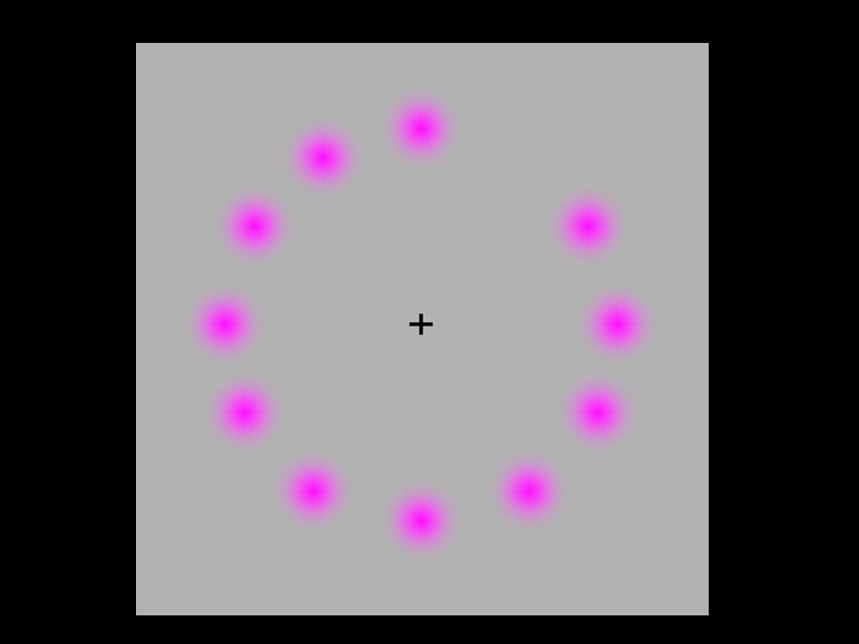
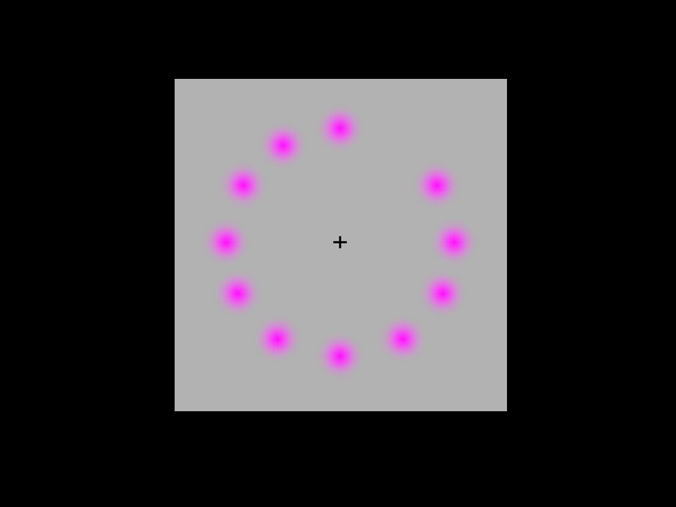
102. Moving Dots Another illusion … Follow the moving dot - see pink dot moving in circle Look at the center cross and the dots appear green Concentrate on center cross and pink dots slowly disappear and only a green dot will be seen rotating Follow the “space” and all seems to be rotating (maybe) “Blink” (redirect eyes) at any time to stop

105. Afterimage + attentional shift + … “moving dots” Particularly compelling –Again, an illusion is an extreme case – somewhat “surprising” because it leads to error Explained by afterimage, attentional shift, lateral inhibition (last time), … For computer graphics, illusions illustrate: –“things are not always as they appear to be” What is perceived by user is not necessarily what is displayed –Human visual system is complex, but not unknowable Should at least “be sensitive to” challenges and be able to explain –Are both sensory and perceptual mechanisms at work Sensory, –Here, afterimage – just bleached pigments Perceptual –Here, shifting attention and inhibition

106. End.