2. Implementation of Hull- White´s No-Arbitrage Term Structure Model Copyright, 1998 © Eugen Puschkarski Diploma Thesis of Eugen Puschkarski

3. Introduction Some preliminary definitions Overview of term structure models Tree building procedure Applications, Convergence behavior Volatility parameter estimation, Calibration Hedge parameters That’s it

4. Some preliminary definitions Risk-neutral pricing No-Arbitrage requirement

5. p<1 risk neutral probability P(t,  )/B(t,  ) follows a martingale = its expected future value equals its current value

6. market is frictionless no taxes or transaction costs securities are perfectly divisible bond market is complete there exists a discount bond for each maturity Assumptions of risk neutral pricing

7. Relation to Arrow-Debreu prices

8. Overview of Interest Rate Models Three ways to model the term structure Assuming (modeling) a stochastic process for discount bond prices instantaneous forward rates short rate internal rate of return of a discount bond with infinitesimally short period of time to maturity

9. Equilibrium Term Structure Models term structure of interest rates as an output given some assumptions about how an overall economic equilibrium is achieved

10. Rendleman and Bartter builds on Cox, Ross and Rubinstein’s binomial representation of a stock price following geometric Brownian motion does not allow negative interest rates easy to implement

11. Vasicek assumes that the short rate follows a Markov process and that the bond price P at time t with maturity  is determined by the short rate process in this time interval

12. Since the price of the bond is only dependent on one stochastic variable r these kind of models are called one factor models. By applying Itos Lemma, Vasicek derives the differential equation for any discount bond P as

13. is called the market price of risk of r and is equal to with  and  as the expected return and volatility of P

14. a, b and s are constants short rate reverts to its long-run mean b at rate a this is called mean reversion Vasicek assumes the process for the short rate to be

15. By solving the differencial equation with regard to the short rate process and subject to the boundary condition P( ,  )=1 Vasicek presents the price of a discount bond as

16. Term Structure is then given by the short rate is normally distributed so negative interest rates can occur because of mean reversion the probability for negative rates should be small

17. Cox, Ingersoll and Ross specify only one factor determining the interest rates namely the short rate which follows the volatility of r is proportional to which prevents r to become negative

18. Two Factor Models more flexibility allows the term structure not only to shift up and down but also twist

19. Brennan and Schwartz define the second factor to be the long rate l, which is the yield of a perpetual discount bond

20. Longstaff and Schwartz use the general equilibrium framework of Cox, Ingersoll and Ross assume two independent unspecified state variables (factors)

21. Using the fundamental partial differential equation for interest rate contingent claims dependent on two factors developed by Cox, Ingersoll and Ross it is possible to determine the short rate r and its instantaneous variance V as part of the equilibrium

22. No-Arbitage Term Structure Models no-arbitrage term structure models take the initial term structure as an input by using time-varying parameters procedure of adjusting parameters so that the initial term structure is exactly matched is generally called calibrating

23. Ho and Lee model the discrete evolution of bond prices by specifying perturbation functions continuous time version of the Ho and Lee model can be represented by a model of the short rate

24. with time varying mean of dr F t (0,t) denotes the partial derivative of the initial instantaneous forward rate with respect to t

25. Properties r(t) is Markov which is equivalent to a constant volatility of forward rates short rate r can be represented by a recombining binomial tree model incorporates no mean reversion interest rates can become negative

26. Hull-White an extension of Ho and Lee as it allows mean reversion an extension of Vasicek as it is a no- arbitrage model

27. At any time t the short rate r reverts to at rate a when a=0 the Hull and White model reduces to the Ho and Lee model bond prices can be calculated at any time t from

28. Heath, Jarrow, and Morton built a term structure model of a general type by modeling the instantaneous forward rate showed that there exists a link between the drift and standard deviation of this instantaneous forward rate it is sufficient to know the standard deviations to construct a term structure model

29. allowing for k factors to influence the instantaneous forward rate F(t,T) The link between drift m(t,T) and standard deviations s k (t,T) is given by

30. One specific version with two factors has become known as the Heath, Jarrow, and Morton model lognormal model (non-negative interest rates) allows for parallel shifts and twists in the term structure

31. does generally not allow to be represented in a recombining tree as the forward rate and therefore the short rate are non-Markov Only by restricting the volatility of bond prices not to be stochastic Markov models for the short rate can be constructed.

32. Ho and Lee model assumes a bond price volatility of and Hull and White of

33. these models can be constructed by a recombining tree it is computationally easier and faster to implement a recombining tree than a path-dependent tree which requires in most cases the use of Monte Carlo simulation.

34. Matching the volatility term structure of interest rates other time-varying parameters have been added to the short rate process in order to give it enough degrees of freedom to match also the term structure of volatilities exactly has the drawback that the resulting future volatility term structure is often quite different from the initially observed one

35. Black, Derman, and Toy use a binomial tree with constant local probabilities (p u =p d =0.5) and time steps to match the twofold term structure by a trial and error procedure forward induction or the analytic approximation tree building procedure of Bjerksund and Stensland (1996) are to be preferred

36. continuous process of the short rate is the speed of mean reversion and the short rate volatility are time-dependent Short rates are lognormally distributed

37. Black and Karasinski more general model by making the speed of mean reversion independent of the volatility of interest rates but preserving its time- dependent feature use time steps of varying lengths three different time-varying parameters lognormal Hull-White model with a time dependent a and .

38. Tree building procedure Hull-White choose to represent the evolution of r by a trinomial tree because it gives the model enough freedom to match the expected value and variance of  r

39. First an auxiliary tree for the process is constructed To calculate the probabilities of each branch in the tree we consider to match the expected change and variance in r over a time interval  t.

40. probabilities must also sum to unity gives us three equations in the three probabilities p u, p m and p d Hull-White suggest to choose  r to be

41. expected change in r equals Type AType B

42. Type C

43. Now that the initial tree is built, it is necessary to displace the nodes at time i  t by  i which is calculated to produce bond prices consistent with the initial term structure.

44. Applying forward induction

45. More generally The summation is taken over all values of k for which the probability is nonzero.

46. Applications Discount bond options analytical solution

47. Numerical solution

48. Example European put bond option on a 9 year zero coupon bond face value 100 time to maturity of 3 years a=0.1 and  =0.01

49. Term Structure strike price is set to the three year forward price of the bond

50. Results

51. Convergence analysis

54. more exact results for at-the-money and in-the-money options Therefore we recommend using at least 150 time steps for out-of-the- money options and about 50 for all other options.

55. Computation time

56. American options will never be optimal to exercise an American call option on discount bonds! will always be optimal to exercise an American put option on discount bonds! immediately

57. Coupon bond options portfolio of discount bond options

58. Floaters non-standard floating rate bonds interval between interest payments is not equal to the term of the floating rate

59. Caps, Floors, Collars A cap provides a payment everytime a specified floating rate like the 6 month LIBOR exceeds the agreed cap rate. individual payments are called caplets and as a sum make up a cap reference rate is observed at the beginning of the period starting at t=1 and eventually a payment is made at the end of the period

60. we have to calculate the cash flows at the time the reference rate is measured which is at the beginning of the period Caplet as a put option with maturity at the beginning of the considered period and strike price L on a discount bond which matures at the end of the period and face value

61. term of the reference rate k does not match the payment period  A collar is simply a combination of a long position in a cap and a short position in a floor and is calculated accordingly.

62. Example

63. Swaptions Replicating approach option on a payer swap replicated by a put option on the fixed rate coupon bond with strike price equal to the principal Example: 3*6 swaption semiannual payments RcX=0.06 replicated by an option on a coupon bond with 12 coupon payments of and principal L

64. Numerical procedure calculate all possible cash flows at option expiration with

65. Results

66. Accrual Swaps interest on one side accrues only if the floating rate is in a certain range or above or below a rate can be replicated by an ordinary swap and a series of binary options

67. Example fixed rate accrues only if the 3-month LIBOR is below RcX=0.08 cont. Comp swap pays every three month for 9 months time

68. Callable, Putable Bonds callable bond for example gives the issuer the right to call the bonds at certain times or at any time at a prespecified price putable bond gives the holder the right of early redemption calculate terminal value of the bond work backward by change min to max if putable

69. Example Discount bond with 9 years to maturity

70. Volatility parameter estimation two volatility parameters a and   : absolute volatility of the short rate a: gives the relative volatility of the long and short rates volatility of the zero rate with maturity T

71. volatility parameters are not directly provided by the market have to be inferred from market data of interest rate derivatives

72. Example infer the volatility parameters from Caps and Floors on the DEM 6 month LIBOR rate different strike rates and time to maturity actively traded and their model prices can be calculated analytically

73. Term Structure for DEM as of 4/8/1998

74. Cap and Floor prices

75. Results

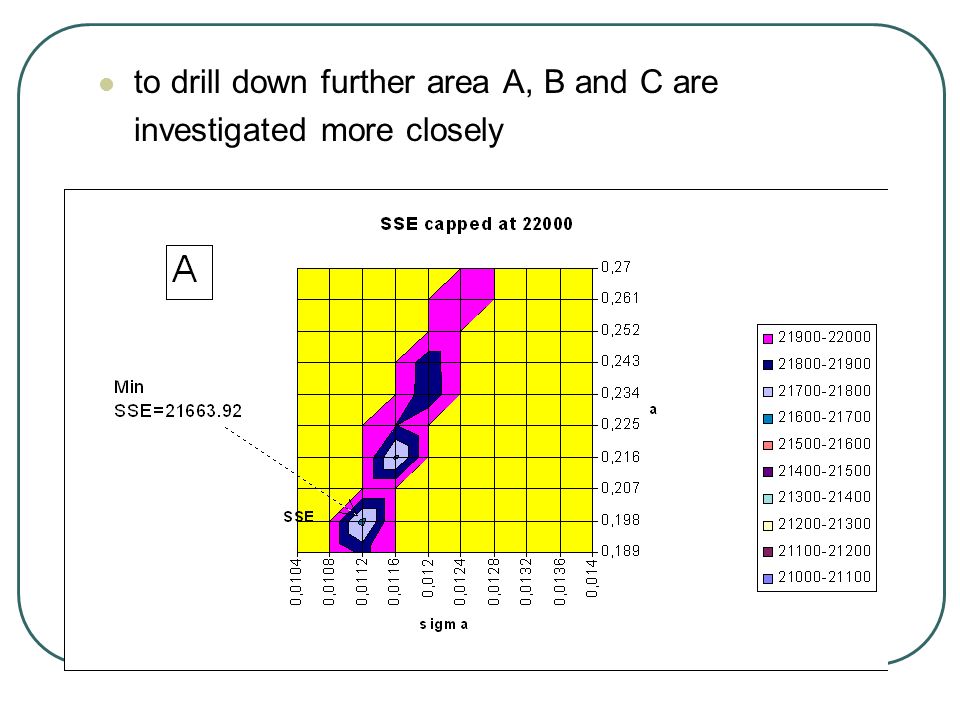
76. Another procedure: calculate a 10*10 matrix of SSE values for 10 different equally spaced values of a and 

77. Calculate a new 10*10 matrix within the new borders of a and .

79. to drill down further area A, B and C are investigated more closely

81. the solution for the optimal a and  which the solver provides seems to be the correct one since it lies in area A which shows the minimum SSE of all areas considered

82. Hedge parameters Delta Gamma

83. new derivative values for the shifted yield curve can be approximated by a Taylor series expansion like

84. Twists calculate delta by dividing the change in the value of the derivative by the tenor weighted sum of the individual shifts

86. Bucket shifts we can approximate any shift as a series of bucket shifts give an example of a three year discount bond option on a 9 year bond

87. Shift of volatility parameters hedge parameters of first order a_vega sigma_vega second order hedge parameters a_vega2 sigma_vega2 shift of a in 0.01 steps and of  in 0.001 steps

89. Conculding remarks Hull-White model is a very flexible model allowing the user to either use an analytical or numerical solution mean reverting feature no-arbitrage property is a one factor model whereas at least three factors driving interest rates have been identified at the time of writing no dominant term structure model has emerged