1. Rule Generation
[Chapter ]
Given a frequent itemset L, find all non-empty subsets f  L such that f  L – f satisfies the minimum confidence requirement
If {A,B,C,D} is a frequent itemset, candidate rules:
ABC D, ABD C, ACD B, BCD A, A BCD, B ACD, C ABD, D ABC AB CD, AC  BD, AD  BC, BC AD, BD AC, CD AB,
If |L| = k, then there are 2k – 2 candidate association rules (ignoring L   and   L)

2. Rule Generation
How to efficiently generate rules from frequent itemsets?
In general, confidence does not have an anti- monotone property
c(ABC D) can be larger or smaller than c(AB D)
But confidence of rules generated from the same itemset has an anti-monotone property
e.g., L = {A,B,C,D}: c(ABC  D)  c(AB  CD)  c(A  BCD)
Confidence is anti-monotone w.r.t. number of items on the RHS of the rule

3. Rule Generation for Apriori Algorithm
[optional]
Lattice of rules
Pruned Rules
Low Confidence Rule

4. Rule Generation for Apriori Algorithm
[optional]
Candidate rule is generated by merging two rules that share the same prefix in the rule consequent
join(CD=>AB,BD=>AC) would produce the candidate rule D => ABC
Prune rule D=>ABC if its subset AD=>BC does not have high confidence

5. Midterm Exam 1
(d) List all association rules with the minimum confidence minconf=50% and minimum support minsup=30%.
Transaction ID
Items Bought 1
{a,b,d,e} 2
{b,c,d} 3 4
{a,c,e} 5
{b,c,d,e} 6
{b,d } 7
{c,d} 8
{a,b,c} 9
{a,d,e} 10
{b,e}

6. F F F F F F F F F F F F F F F F

7. ab, ad, ae, bc, bd, be, cd, de, ade, bde
Transaction ID
Items Bought 1
{a,b,d,e} 2
{b,c,d} 3 4
{a,c,e} 5
{b,c,d,e} 6
{b,d } 7
{c,d} 8
{a,b,c} 9
{a,d,e} 10
{b,e}
ade->{ }
de->a
ae->d
ad->e
e->ad
d->ae
a->de

8. Midterm 4.
(a) Build a decision tree on the data set by using misclassification error rate as the criterion for splitting.
(b) Build the cost matrix and a new decision tree accordingly.
(c) What are the accuracy, precision, recall, and F1- measure of the new decision tree?

9. x y Error rate =260/640*10/260+360/640*10/360 =20/640 Error rate- 10
250 1 20 2
350
Error rate
=260/640*10/ /640*10/360
=20/640 y + -
250 1 40
150 2
200
Error rate
=190/640*40/190
=40/640

10. x x + - 10
250 1 20 2
350 2 1 y 1 2 + 1 2 y
(X=2) y + -
150 1 10
100 2 - -
(X=0) y + -
100 1 10 50 2 x 1
0,2 + -

11. - - + x y + predicted real 2 1 + ? or + - 2*600/40=30 3 (X=0) y + -
2*600/40=30 3
real x 1 2 + y ?
(X=0) y + -
100 1 10 50 2
10*0+50*3=150
10*30+50*0=300
(X=2) y + -
150 1 10
100 2 - - +
10*0+100*3=300
10*30+100*0
=300 or +

12. - + - x y a b c d 2 1 + ? accuracy=(30+450)/640 Recall=30/(30+10)2 + y ? x + - 10
250 1 20 2
350
(X=2) y + -
150 1 10
100 2
(X=0) y + -
100 1 10 50 2 - + - + - 30 10 50
450 a b c d
accuracy=(30+450)/640
Precision=30/(30+50)
Recall=30/(30+10)
F-measure=2*30/(2* )

13. Bayesian Theorem
Given training data X, posteriori probability of a hypothesis H, P(H|X) follows the Bayes theorem
Informally, this can be written as
posterior =likelihood x prior / evidence
Predicts X belongs to C2 iff the probability P(Ci|X) is the highest among all the P(Ck|X) for all the k classes
Practical difficulty: require initial knowledge of many probabilities, significant computational cost

14. Naïve Bayes Classifier
A simplified assumption: attributes are conditionally independent and each data sample has n attributes
No dependence relation between attributes
By Bayes theorem,
As P(X) is constant for all classes, assign X to the class with maximum P(X|Ci)*P(Ci)

15. Bayesian Networks
Bayesian belief network allows a subset of the variables conditionally independent
A graphical model of causal relationships
Represents dependency among the variables
Gives a specification of joint probability distribution
Nodes: random variables
Links: dependency
X,Y are the parents of Z, and Y is the parent of P
No dependency between Z and P
Has no loops or cycles Y Z P
Casual X

16. Bayesian Belief Network: An Example
One conditional probability table (CPT) for each variable
The CPT for the variable LungCancer:
Shows the conditional probability for each possible combination of its parents
Family
History
LungCancer
PositiveXRay
Smoker
Emphysema
Dyspnea
(FH, S)
(FH, ~S)
(~FH, S)
(~FH, ~S) LC
~LC
0.8
0.2
0.5
0.7
0.3
0.1
0.9
Derivation of the probability of a particular combination of values of X, from CPT:
Bayesian Belief Networks

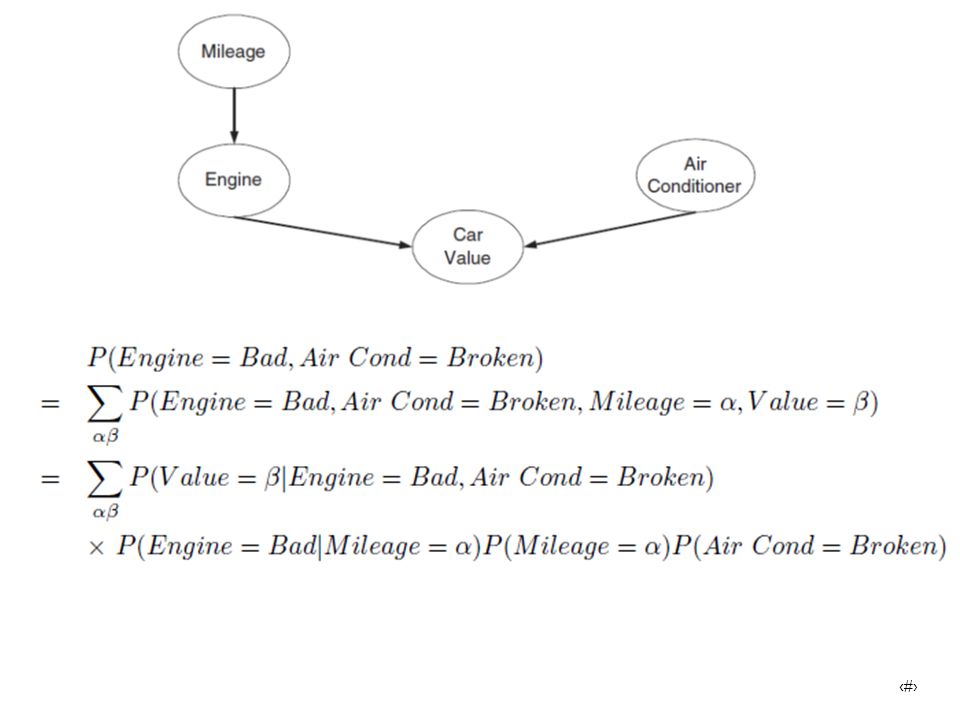
17. Midterm Exam 5
(a) Draw the probability table for each node in the network.
(b) Use the Bayesian network to compute P(Engine = Bad, Air Conditioner= Broken).
Mileage
Engine
Air Conditioner
Number of Records
with Car Value=Hi
with Car Value=Lo Hi
Good
Working 3 4
Broken 1 2
Bad 5 Lo 10
由於貝氏定理可以結合事前機率與樣本機率，比較一般利用統計方法來說，貝氏定理能更有效的運用有限的樣本    資訊與經驗值，所以再分析資料時不需太多的樣本資訊就可得到理想的統計數值，進而做更有效率的推論。貝氏    網路其型態為圖形模式，可說明變數間的機率關係。圖形模式結合統計方法後，很適合運用在資料分析問題。貝    氏網路具有下列三項優點：         ‧貝氏網路可以輕易地處理不完整的資料，且貝氏網路提供了一個表示相依關係的知識表示法。    ‧貝氏網路允許因果關係的學習。    ‧貝氏網路透過貝氏統計的方法，可以將領域知識與資料之間做結合。

18. P(C=Hi|E=G,A=W))=13/17 P(C=Lo|E=G,A=W))=4/17 P(M=Hi)= 0.5
Mileage
Engine
Air Conditioner
Number of Records
with Car Value=Hi
with Car Value=Lo Hi
Good
Working 3 4
Broken 1 2
Bad 5 Lo 10
P(C=Hi|E=G,A=W))=13/17
P(C=Lo|E=G,A=W))=4/17
P(C=Hi|E=G,A=B)=4/7
P(C=Lo|E=G,A=B)=3/7
P(C=Hi|E=B,A=W)=0.3
P(C=Lo|E=B,A=W)=0.7
P(C=Hi|E=B,A=B)=0
P(C=Lo|E=B,A=B)=1
P(M=Hi)= 0.5
P(M=Lo)= 0.5
P(M=Hi)= 20/40=0.5
P(A=W)= ( )/40=27/40
P(A=B)= ( )/40=13/40
P(E=G|M=Hi)= ( )/( )=10/20=0.5
P(E=B|M=Hi)= (1+5+4)/( )=10/20=0.5
P(E=G|M=Lo)= ( )/( )=14/20=0.7
P(E=B|M=Lo)= (2+2+2)/( )=6/20=0.3
P(C=Hi|E=G,A=W))=(3+10)/(3+4+10)=13/17
P(C=Lo|E=G,A=W))=(4)/(3+4+10)=13/17
P(C=Hi|E=G,A=B)=(1+3)/( )=4/7
P(C=Lo|E=G,A=B)=(2+1)/( )=3/7
P(C=Hi|E=B,A=W)=(1+2)/( )=3/10=0.3
P(C=Lo|E=B,A=W)=(5+2)/( )=0.7
P(C=Hi|E=B,A=B)=0/(4+2)=0
P(C=Lo|E=B,A=B) =(4+2)/(4+2)=1
P(A=W)= 27/40
P(A=B)= 13/40
P(E=G|M=Hi)= 0.5
P(E=B|M=Hi)=0.5
P(E=G|M=Lo)= 0.7
P(E=B|M=Lo)= 0.3