1. Topic 28: Unequal Replication in Two-Way ANOVA

2. Outline Two-way ANOVA with unequal numbers of observations in the cells –Data and model –Regression approach –Parameter estimates Previous analyses with constant n just special case

3. Data for two-way ANOVA Y is the response variable Factor A with levels i = 1 to a Factor B with levels j = 1 to b Y ijk is the k th observation in cell (i,j) k = 1 to n ij and n ij may vary

4. Recall Bread Example KNNL p 833 Y is the number of cases of bread sold A is the height of the shelf display, a=3 levels: bottom, middle, top B is the width of the shelf display, b=2: regular, wide n=2 stores for each of the 3x2 treatment combinations (BALANCED)

5. Regression Approach Create a-1 dummy variables to represent levels of A Create b-1 dummy variables to represent levels of B Multiply each of the a-1 variables with b-1 variables for B to get variables for AB LET’S LOOK AT THE RELATIONSHIP AMONG THESE SETS OF VARIABLES

6. Common Set of Variables data a2; set a1; X1 = (height eq 1) - (height eq 3); X2 = (height eq 2) - (height eq 3); X3 = (width eq 1) - (width eq 2); X13 = X1*X3; X23 = X2*X3;

7. Run Proc Reg proc reg data=a2; model sales= X1 X2 X3 X13 X23 / XPX I; height: test X1, X2; width: test X3; interaction: test X13, X23; run;

8. X′X Matrix Model Crossproducts X'X X'Y Y'Y VariableInterceptX1X2X3X13X23 Intercept1200000 X1084000 X2048000 X30001200 X13000084 X23000048 Sets of variables orthogonal Cross- products between sets is 0

9. Orthogonal X’s Order in which the variables are fit in the model does not matter –Type I SS = Type III SS Order of fit not mattering is true for all choices of restrictions when n ij is constant Orthogonality lost when n ij are not constant

10. KNNL Example KNNL p 954 Y is the change in growth rates for children after a treatment A is gender, a=2 levels: male, female B is bone development, b=3 levels: severely, moderately, or mildly depressed n ij =3, 2, 2, 1, 3, 3 children in the groups

11. Read and check the data data a3; infile 'c:\...\CH23TA01.txt'; input growth gender bone; proc print data=a1; run;

12. Obs growth gender bone 1 1.4 1 1 2 2.4 1 1 3 2.2 1 1 4 2.1 1 2 5 1.7 1 2 6 0.7 1 3 7 1.1 1 3 8 2.4 2 1 9 2.5 2 2 10 1.8 2 2 11 2.0 2 2 12 0.5 2 3 13 0.9 2 3 14 1.3 2 3

13. Common Set of Variables data a3; set a3; X1 = (bone eq 1) - (bone eq 3); X2 = (bone eq 2) - (bone eq 3); X3 = (gender eq 1) - (gender eq 2); X13 = X1*X3; X23 = X2*X3;

14. Run Proc Reg proc reg data=a3; model growth= X1 X2 X3 X13 X23 / XPX I; run;

15. X′X Matrix Model Crossproducts X'X X'Y Y'Y VariableInterceptX1X2X3X13X23 Intercept140030 X19531 X205100-2 X3030140 X1331 95 X230-20510 Cross- product terms no longer 0 Order of fit matters

16. How does this impact the analysis? In regression, this happens all the time (explanatory variables are correlated) –t tests look at significance of variable when fitted last When looking at comparing means order of fit will alter null hypothesis

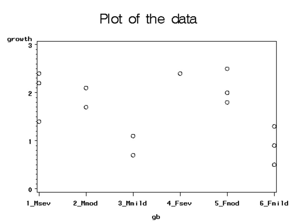
17. Prepare the data for a plot data a1; set a1; if (gender eq 1)*(bone eq 1) then gb='1_Msev '; if (gender eq 1)*(bone eq 2) then gb='2_Mmod '; if (gender eq 1)*(bone eq 3) then gb='3_Mmild'; if (gender eq 2)*(bone eq 1) then gb='4_Fsev '; if (gender eq 2)*(bone eq 2) then gb='5_Fmod '; if (gender eq 2)*(bone eq 3) then gb='6_Fmild';

18. Plot the data title1 'Plot of the data'; symbol1 v=circle i=none; proc gplot data=a1; plot growth*gb; run;

20. Find the means proc means data=a1; output out=a2 mean=avgrowth; by gender bone; run;

21. Plot the means title1 'Plot of the means'; symbol1 v='M' i=join c=blue; symbol2 v='F' i=join c=green; proc gplot data=a2; plot avgrowth*bone=gender; run;

22. Interaction?

23. Cell means model Y ijk = μ ij + ε ijk –where μ ij is the theoretical mean or expected value of all observations in cell (i,j) –the ε ijk are iid N(0, σ 2 ) –Y ijk ~ N(μ ij, σ 2 ), independent

24. Estimates Estimate μ ij by the mean of the observations in cell (i,j), For each (i,j) combination, we can get an estimate of the variance We pool these to get an estimate of σ 2

25. Pooled estimate of σ 2 In general we pool the s ij 2, using weights proportional to the df, n ij -1 The pooled estimate is s 2 = (Σ (n ij -1)s ij 2 ) / (Σ(n ij -1)) Nothing different in terms of parameter estimates from balanced design

26. Run proc glm proc glm data=a1; class gender bone; model growth=gender|bone/solution; means gender*bone; run; Shorthand way to write main effects and interactions

27. Parameter Estimates Solution option on the model statement gives parameter estimates for the glm parameterization These constraints are –Last level of main effect is zero –Interaction terms with a or b are zero These reproduce the cell means in the usual way

28. Parameter Estimates ParameterEstimate Standard Errort ValuePr > |t| Intercept0.90000000B0.23273733.870.0048 gender 1-0.00000000B0.3679900-0.001.0000 bone 11.50000000B0.46547473.220.0122 bone 21.20000000B0.32914033.650.0065 gender*bone 1 1-0.40000000B0.5933661-0.670.5192 gender*bone 1 2-0.20000000B0.5204165-0.380.7108

29. Output Note DF and SS add as usual SourceDF Sum of Squares Mean SquareF ValuePr > F Model54.47428570.894857145.510.0172 Error81.30000000.16250000 Corrected Total135.7742857

30. Output Type I SS SSG+SSB+SSGB=4.47429 SourceDFType I SSMean SquareF ValuePr > F gender10.00285710.002857140.020.8978 bone24.39600002.1980000013.530.0027 gender*bone20.07542860.037714290.230.7980

31. Output Type III SS SSG+SSB+SSGB=4.38514 SourceDFType III SSMean SquareF ValuePr > F gender10.12000000 0.740.4152 bone24.189714292.0948571412.890.0031 gender*bone20.075428570.037714290.230.7980

32. Type I vs Type III SS for Type I add up to model SS SS for Type III do not necessarily add up Type I and Type III are the same for the interaction because last term in model The Type I and Type III analysis for the main effects are not necessarily the same Different hypotheses are being examined

33. Type I vs Type III Most people prefer the Type III analysis This can be misleading if the cell sizes differ greatly Contrasts can provide some insight into the differences in hypotheses

34. Contrast for A*B Same for Type I and Type III Null hypothesis is that the profiles are parallel; see plot for interpretation μ 12 - μ 11 = μ 22 - μ 21 and μ 13 - μ 12 = μ 23 - μ 22 μ 11 - μ 12 - μ 21 + μ 22 = 0 and μ 12 - μ 13 - μ 22 + μ 23 = 0

35. A*B Contrast statement contrast 'gender*bone Type I and III' gender*bone 1 -1 0 -1 1 0, gender*bone 0 1 -1 0 -1 1; run;

36. Type III Contrast for gender (1) μ 11 = (1)(μ + α 1 + β 1 + (αβ) 11 ) (1) μ 12 = (1)(μ + α 1 + β 2 + (αβ) 12 ) (1) μ 13 = (1)(μ + α 1 + β 3 + (αβ) 13 ) (-1) μ 21 = (-1)(μ + α 2 + β 1 + (αβ) 21 ) (-1) μ 22 = (-1)(μ + α 2 + β 2 + (αβ) 22 ) (-1) μ 23 = (-1)(μ + α 2 + β 3 + (αβ) 23 ) L = 3α 1 – 3α 2 + (αβ) 11 + (αβ) 12 + (αβ) 13 – (αβ) 21 – (αβ) 22 – αβ 23

37. Contrast statement Gender Type III contrast 'gender Type III' gender 3 -3 gender*bone 1 1 1 -1 -1 -1;

38. Type I Contrast for gender (3) μ 11 = (3)(μ + α 1 + β 1 + (αβ) 11 ) (2) μ 12 = (2)(μ + α 1 + β 2 + (αβ) 12 ) (2) μ 13 = (2)(μ + α 1 + β 3 + (αβ) 13 ) (-1) μ 21 = (-1)(μ + α 2 + β 1 + (αβ) 21 ) (-3) μ 22 = (-3)(μ + α 2 + β 2 + (αβ) 22 ) (-3) μ 23 = (-3)(μ + α 2 + β 3 + (αβ) 23 ) L = (7α 1 – 7α 2 )+(2β 1 – β 2 – β 3 )+3(αβ) 11 +2(αβ) 12 +2(αβ) 13 –1(αβ) 21 –3(αβ) 22 –3(αβ) 23

39. Contrast statement Gender Type I contrast 'gender Type I' gender 7 -7 bone 2 -1 –1 gender*bone 3 2 2 -1 -3 -3;

40. Contrast output Contrast DF Contrast SS gender Type III 1 0.12000000 gender Type I 1 0.00285714 bone Type III 2 4.18971429 gender*bone Type I and III 2 0.07542857

41. Summary Type I and Type III F tests test different null hypotheses Should be aware of the differences Most prefer Type III as it follows logic similar to regression analysis Be wary, however, if the cell sizes vary dramatically

42. Comparing Means If interested in Type III hypotheses, need to use LSMEANS to do comparisons If interested in Type I hypotheses, need to use MEANS to do comparisons. We will show this difference via the ESTIMATE statement

43. SAS Commands Will use earlier contrast code to set up the ESTIMATE commands estimate 'gender Type III' gender 3 -3 gender*bone 1 1 1 -1 -1 -1 / divisor=3; estimate 'gender Type I' gender 7 -7 bone 2 -1 -1 gender*bone 3 2 2 -1 -3 -3 / divisor=7;

44. MEANS OUPUT Level of ------------growth----------- gender N Mean Std Dev 1 7 1.65714286 0.62411843 2 7 1.62857143 0.75655862 Diff = 0.0286

45. LSMEANS OUPUT growth gender LSMEAN 1 1.60000000 2 1.80000000 Diff = -0.20

46. Estimate output Parameter Estimate Std Err gender Type III -0.200 0.2327 gender Type I 0.029 0.2155 Notice that these two estimates agree with the difference of estimates for LSMEANS or MEANS

47. Analytical Strategy First examine interaction Some options when the interaction is significant –Interpret the plot of means –Run A at each level of B and/or B at each level of A –Run as a one-way with ab levels –Use contrasts

48. Analytical Strategy Some options when the interaction is not significant –Use a multiple comparison procedure for the main effects –Use contrasts for main effects –If needed, rerun without the interaction

49. Example continued proc glm data=a3; class gender bone; model growth=gender bone/ solution; means gender bone/ tukey lines; run; Pool here because small df error For Type I hypotheses

50. Output SourceDF Sum of SquaresMean SquareF ValuePr > F Model34.39885711.4662857110.660.0019 Error101.37542860.13754286 Corrected Total135.7742857

51. Output Type I SS SourceDFType I SSMean SquareF ValuePr > F gender10.00285714 0.020.8883 bone24.396000002.1980000015.980.0008

52. Output Type III SS SourceDFType III SSMean SquareF ValuePr > F gender10.09257143 0.670.4311 bone24.396000002.1980000015.980.0008 Although different null hypothesis for gender, both Type I and III tests are not found significant

53. Tukey comparisons Group Mean N bone A 2.1000 4 1 A A 2.0200 5 2 B 0.9000 5 3

54. Tukey Comparisons Why don’t we need a Tukey adjustment for gender? Means statement does provide mean estimates so you know directionality of F test but that is all the statement provides you

55. Last slide Read KNNL Chapter 23 We used program topic28.sas to generate the output for today