1. Medical Imaging Systems: MRI Image Formation
Instructor: Walter F. Block, PhD 1-3
Notes: Walter Block and Frank R Korosec, PhD 2-3
Tuesday 9 August 1994 at 17h36
S.F. Hilton and Towers, Continental question period
Pulse Sequences for Fluid Shear Measurement using Fourier-encoded Velocity Imaging.
Session: Flow Quantification
Chairs: D. Saloner and L. Frank
Departments of Biomedical Engineering 1,
Radiology 2 and Medical Physics 3
University of Wisconsin - Madison

2. But so far RF coils only integrate signal
MRI Physics: So far...
What we can do so far:
1) Excite spins using RF field at o
2) Record time signal (Known as FID)
3) Mxy decays, Mz grows
4) Repeat.
But so far RF coils only integrate signal
from entire body. We have no way of
forming an image. That brings us to the
last of the three magnetic fields in MRI. S?

3. Image Formation Overview
Gradient fundamentals
Slice Selection
Limit excitation to a slice or slab
Can be in any orientation
Gradient echo in-plane spatial encoding
Radial imaging ( like CT)
Frequency encoding
Phase encoding

4. 3nd Magnetic Field Static High Field Radiofrequency Field (RF)
Termed B0
Creates or polarizes signal
1000 Gauss to 100,000 Gauss
Earth’s field is 0.5 G
Radiofrequency Field (RF)
Termed B1
Excites or perturbs signal into a measurable form
O.1 G but in resonant with signal
Gradient Fields
1 -4 G/cm
Used to determine spatial position of signal
MR signal not based directly on geometry

5. Gradient Coils
Fig. Nishimura, MRI Principles

6. X Gradient Example: Gx
Magnetic field all along z, but magnetic strength can varies spatially with x. Stronger at right, no change in middle, weaker at left.

7. Gradient Coil Fundamentals
Gradient strength directly proportional to current in coil
On the order of 100 amps peak
Performance
Power needed proportional to radius5
Tight bore for patient
Strength – G/cm or mT/m
4 G/cm is near peak now for clinical scanners
Higher strength with localized gradients (research only)
Slew rate
Need high voltages to change current quickly
T/m/s is high performance
Rise to 1 G in .1 ms at 100 T/m/s
Limited by peripheral nerve stimulation

8. Magnetic Field Gradient Timing Diagrams

9. B0 (t)(B0 + Gx(t)x) Before, only B0 Now with Gx
Larmor Equation
B0
Before, only B0
Precessional
Frequency
Static Magnetic Field
(t)(B0 + Gx(t)x)
Now with Gx

10. Gx, Gy, Gz: One for each spatial dimension
Magnetic field all along z, but magnetic strength can vary spatially with x, y, and/or z.

11. Two Object Example of Spatial Encoding
sr(t)
Receiver Signal: No gradient
Gx On: Beat Frequency
Demodulated Signal x
m(x)
Water

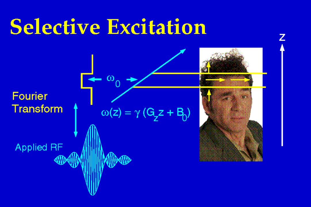
12. Gz Gradient Example
L31, slides repeated here: first imaging method, basic procedure, projection reconstruction.
The effects of the main magnetic field and the applied slice gradient. In this example, the local magnetic field changes in one-Gauss increments accompanied by a change in the precessional frequency from chin to the top of the head.
Image, caption: copyright Proruk & Sawyer, GE Medical Systems Applications Guide, Fig. 11

13. Selective RF Excitation
Recall frequency of RF excitation has to be equal
or in resonance with spins
Build RF pulse from sum of narrow frequency range

14. Frequency profile of modulated RF pulse
Slice Selection
- Consider a pulse B1(t) that is multiplied by cos(ot). This is called modulation .
B1(t) is called the RF excitation.
o is the carrier frequency = g B0.
Mixer
B1(t) cos(ot)
A(t)
cos(ot)
Frequency profile of modulated RF pulse
o = 2fo wo f

16. Frequency Encoding Spin Frequency (x)
Image each voxel along x as a piano key that has a different pitch. MR coil sums the “keys” like your ear.
Fig from Illustrator, mag 100% then shrunk in powerpoint

17. Frequency Encoding

18. GRE Pulse Sequence Timing Diagramrf
Slice
Select
Freq.
Encode
Signal TE

19. Frequency Encoding & Data Sampling
Generated
Signal
DAQ
Sampled
Signal

20. In-plane Encoding
MR signal in frequency encoding (x) is Fourier transform of projection of object
Line integrals along y
Encoding in other direction
Vary angle of frequency encoding direction
1D FT along each angle and Reconstruct similar to CT
Apply sinusoidal weightings along y direction
Spin-warp imaging or phase-encoding
By far the most popular

21. 2D Projection Reconstruction MRIky  kx Gx Gy
DAQ
Reconstruction: convolution back projection or filtered back projection

22. Central Section Theorem in MRI
Object y’ y
In MR, echo gives a radial line in spatial frequency space (k-space). x’ ky θ x θ x’ kx
F.T.
CT Projection
MR Signal (t)
Interesting - Time signal gives spatial frequency information of m(x,y)

23. k-Space Acquisition (Radial Sampling)
Y readout
X readout ky kx kx ky

24. In-plane Encoding
MR signal in frequency encoding (x) is Fourier transform of projection of object
Line integrals along y
Encoding in other direction
Vary angle of frequency encoding direction
1D FT along each angle and Reconstruct similar to CT
Apply sinusoidal weightings along y direction
Apply prior to frequency encoding
Repeat several times with different sinusoidal weightings
Spin-warp imaging or phase-encoding
By far the most popular

25. Phase Encoding: Apply Gy before Freq. encoding
Fig from Illustrator, mag 130%

26. GRE Pulse Sequence Timing Diagramrf
Slice
Select
Phase
Encode
Freq.
Encode
Signal TE

27. k-Space Acquisition ky kx Phase Direction One line of k-space
Encode
Sampled
Signal
DAQ kx ky
Phase
Direction
One line of k-space
acquired per TR
Frequency Direction

28. k-Space Signal ky kx

29. 512 x 512
8 x 8

30. 512 x 512
16 x 16

31. 512 x 512
32 x 32

32. 512 x 512
64 x 64

33. 512 x 512
128 x 128

34. 512 x 512
256 x 256

35. 512 x 512
512 x 32

36. Scan Duration
Scan Time = TR  PE  NEX
TR = Repetition Time
PE = Number of phase encoding values
NEX = Number of excitations (averages)

37. GRE Pulse Sequence Timing Diagramrf
Slice
Select
Phase
Encode
Freq.
Encode
Signal TE

38. Images of the Knee
-weighted
T2-weighted
Needs longer TE

39. T2 & T2* Relaxation: Sources of Image Contrast
Mxy
T2*
Time
T2* 1 = T2 +
B0

40. Effects of Local Magnetic Inhomogeneity
6GRADECH.AVI
The location or phase of spins throughout the x,y plane The first time point shows the spins immediately after the RF pulse.
In the left plot, no gradient is played. In the right plot, the gradient waveform has equal positive and negative areas.
The marker on top labeled “MAG1” or “MAG2” gives the magnitude of the signal in each case.
In the left plot, a local magnetic field distortion is present that causes the
vectors to become dephased naturally and the vector sum of the vectors to become smaller over
time (T2* decay). This dephasing can be observed over a period of 16 frames in the vector plot
on the left. The vector sum of the magnetization vectors during T2* decay is indicated by
MAG1. On the right is shown the same distribution of magnetization vectors in the same local
field distortion, but with the addition of an applied magnetic field gradient along the x-direction.
The vector sum of the magnetization vectors with this additional dephasing is indicated by
MAG2. The additional dephasing caused by this gradient can be seen by comparing the left and
right vector-field plots, as well as by comparing MAG1 and MAG2. After 8 frames, the field
gradient is reversed. This can be seen by observing the behavior of the vectors in the bottom-
most row on the right. As well, the value of MAG2 begins to increase. The reversed gradient
undoes the dephasing of the originally applied gradient so that, after 16 frames, the vector field
plots and their sums are equal. As shown here, a gradient echo does not restore the signal decay
caused by field inhomogeneities or other sources of dephasing. It merely corrects its own effects.In the left plot, spins dephase due to a magnetic field inhomogeneity.
Gx(t)

41. Perils of Gradient Echo Imaging and T2*
TE = 8 ms
TE = 24 ms
0.17 T GE Orthopedic Scanner

42. Image Formation Overview
Gradient fundamentals
Slice Selection
Limit excitation to a slice or slab
Can be in any orientation
Gradient echo in-plane spatial encoding
Radial imaging
Frequency encoding
Phase encoding

43. T1-, T2-, and Density-Weighted Images
T1_brain_w_tumor.tif, t2_brain_w_tumor.tif, density_brain_w_tumor.tif
From wesolak, janet, series 2, image 16, series 3, image 38, series 3, image 37
T1-weighted
T2-weighted
r-weighted

44. T2-Weighted Image of the Spine

45. Images of the Knee
-weighted
T2-weighted

46. T1-, T2-, and Density-Weighted Images
T1_brain_w_tumor.tif, t2_brain_w_tumor.tif, density_brain_w_tumor.tif
From wesolak, janet, series 2, image 16, series 3, image 38, series 3, image 37
T1-weighted
T2-weighted
r-weighted

47. Spin Echo Parameters TR TE T1-weighting short (400 msec)
long (3000 msec)
long (100 msec)
-weighting

48. Signal vs Weighting T1-weighting long T1, small signal
T1-weighted
T2-weighted
r-weighted
T1-weighting
long T1, small signal
short T1, large signal
T2-weighting
long T2, large signal
short T2, small signal
-weighting
high , large signal
low , small signal