1. Linear Recurrence Relations in Music By Chris Hall

2. The Aim of My Project The goal was to take a composition by Beethoven and generate a linear recurrence relation that best represents the tonality of the music. Sonata No. 1, Op. 12 in D Major

3. Linear Recurrence Relations x n = a 1 x n-1 + a 2 x n-2 + … + a k x n-k

4. Premises only the melodic line was used; no chords. This allows the counting of only a single note at a time. The range of notes used was restricted to the audible range as determined by MIDI: Z 128. The value of a single note was determined by MIDI format with middle C being 60. All notes were sequentially valued based on their pitch relative to the pitch of the notes immediately above and below (i.e. if E is 20, D# is 19 and F is 21).

5. What was investigated The degree of the recurrence relation The range for coefficients The best algorithm for finding the relation The best-fit solution

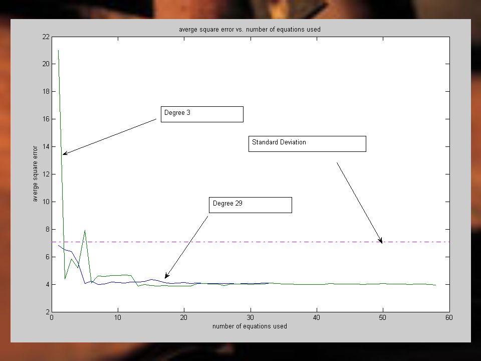
6. Establishing the quality of results The standard deviation of the original set of notes was considered the maximum allowable error for the notes being generated by the relation. The calculated errors considered for comparison were the square errors of the generated notes from the original notes. The average square error of all the notes generated was then compared to the standard deviation of the original note set. Only those errors below the standard deviation were considered acceptable. The highest quality results were considered to be acceptable results with the farthest distance from the standard deviation.

7. The Method The first avenue taken was to consider the same number of equations as unknowns, where the unknowns were the coefficients of the recurrence relation. Like all following methods, MATLAB was used to generate notes, errors and comparisons. The MATLAB program was written to allow the user to enter in their desired degree of relation (which corresponds to the number of unknowns). For the sake of comparison, more than one degree could be entered at a time. The program then produces a series of average square errors on a graph that correspond to the number of equations used, the theory behind which will be discussed a bit later.

8. The First Program

10. Using more equations In order to vary the number of equations used, the least squares method was used. Because the rank of each matrix was full, a unique solution could be obtained. Moreover, since the function considered was the sum of the square errors, the Hessian Matrix of the function was always a multiple of the product of the matrix with its transpose.

11. A simple 4x2 example

12. Other definitive information I know that the point zero is a local minimum because the Hessian Matrix of my original function is positive definite.

13. The Discreet Case The next path for investigation was to analyze coefficients with discreet rather than continuous ranges. It should be noted that these ranges included but were not limited to finite fields. Since the notes themselves were elements of finite range (remember, Z 128 ) the ranges for the coefficient vectors investigated were covered by the range of the notes

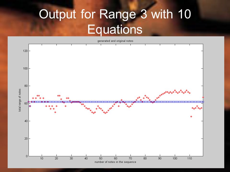
14. The Discreet Case cont’d Another MATLAB program was written that allowed the user to input a desired range of coefficients and the desired number of equations. For reasons to be discussed shortly, only degrees two and three were used. In the degree two case, the square errors were calculated in arrays for all possible combinations of the range of coefficients and then stored in a square matrix that was Range(C)xRange(C) for comparison. The output is the coefficient vector along with the least square error. A graph is also generated that compares the original note set along the total number of notes use with the generated notes. The difference in the degree three case was in the storage of the square errors. In this case, three dimensional storage was required.

15. The Discreet Program

16. Output for Range 3 with 10 Equations

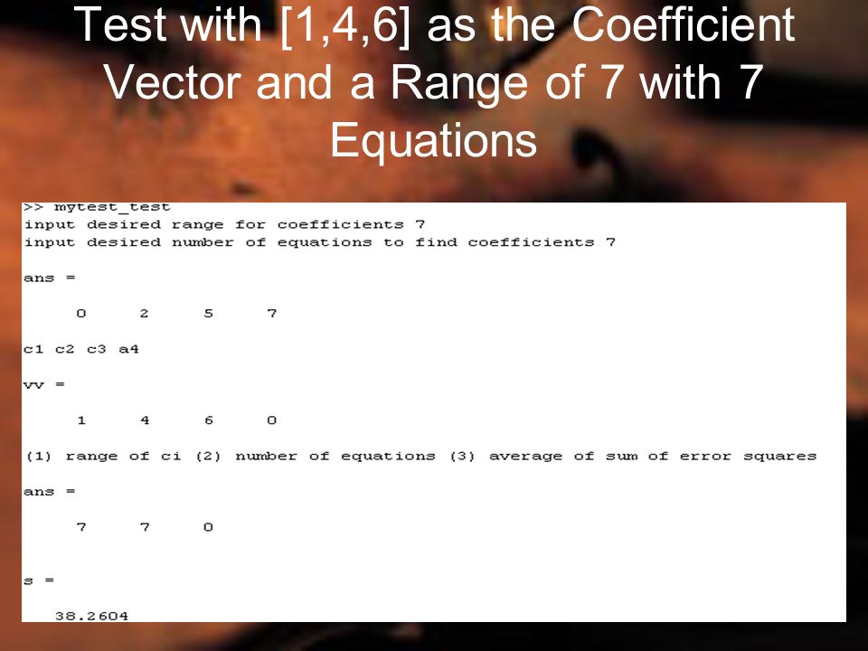
18. Testing With an Actual Recurrence Relation An actual recurrence relation was written to test the program. When the chosen range covered the range of the original coefficients, the program generated the sequence exactly. Otherwise, it produced a best approximation.

19. Test with [1,4,6] as the Coefficient Vector and a Range of 5 with 7 Equations

20. Test with [1,4,6] as the Coefficient Vector and a Range of 7 with 7 Equations

22. Future Work For more discreet analysis, writing a MATLAB program that allows for the continual expansion of the degree should be done. Applying the same methods to other, perhaps less complex, pieces of music (portions of Pachelbel’s Cannon in D Major, for instance). For musical analysis, writing a MATLAB program that would export the generated notes, replacing the originals in the original MIDI file. We might not be producing Beethoven, but it might still be musically interesting.

23. References Steven J. Leon, Linear Algebra With Applications. 7 ed. pp.51, 382-383,234-244 (2006). C.W. Groetsch and J. Thomas King, Matrix Methods & Applications. pp.115-118, 283 (1988). Carla D. Martin, PhD, James Madison University. Ken Schutte, Massachusetts Institute of Technology Mei Chen, PhD, The Military College of South Carolina