1. Climate models, downscaling and uncertainties
Hans von Storch,
GKSS Research Centre, Geesthacht, and
KlimaCampus „clisap“, University of Hamburg Germany
The concept of climate simulations with quasi-realistic climate models is discussed and illustrated with examples. The relevant problem of deriving regional and local specifications is considered as well.

2. Who is this? Hans von Storch (born 1949)
Diploma in mathematics, PhD in meteorology
Director of Institute for Coastal Research, GKSS Research Center, near Hamburg,
Professor at the Meteorological Institute, KlimaCampus, University of Hamburg
Works also with social and cultural scientists.

3. Overview: Quasi-realistic climate models („surrogate reality“)
Free simulations and forced simulations for reconstruction of historical climate
Climate change simulations
Downscaling - Regional climate modelling
Regional scenarios

4. Models as surrogate reality
dynamical, process-based models, • experimentation tool (test of hypotheses) • design of scenario • sensitivity analysis • dynamically consistent interpretation and extrapolation of observations in space and time (“data assimilation”) • forecast of detailed development (e.g. weather forecast)
characteristics: complexity quasi-realistic mathematical/mechanistic engineering approach

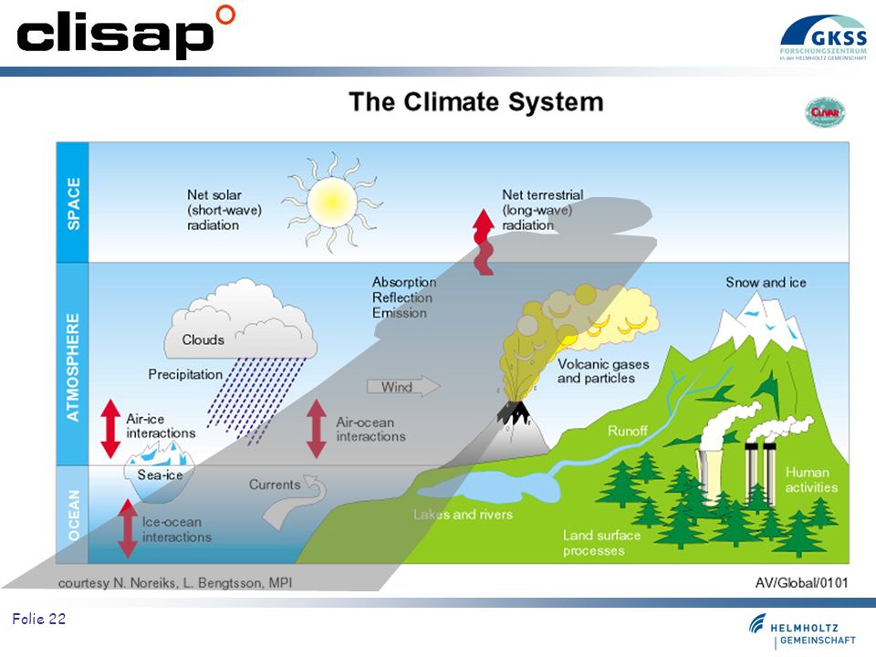
5. Components of the climate system. (Hasselmann, 1995)

6. Quasi-realistic climate models …
… are dynamical models, featuring discretized equations of the type
with state variables Ψk and processes Pi,k.
The state variables are typically temperature of the air or the ocean, salinity and humidity, wind and current.
… because of the limited resolution, the equations are not closed but must be closed by “parameterizations”, which represent educated estimates of the expected effect of non-described processes on the resolved dynamics, conditioned by the resolved state.

7. atmosphere

8. Dynamical processes in the atmosphere

9. Dynamical processes in a global atmospheric general circulation model

10. Results of a survey among climate modellers in 1996, 2003 and 2008
Bray and von Storch, 2010
Results of a survey among climate modellers in 1996, 2003 and 2008

11. Klimazonen Klassifikation nach Koeppen Modell Beobachtet
Erich Roeckner, pers. Mitteilung 11

12. Zyklogenese Sturmbahn-dichten Observed Winter Simulated (DJF)
Erich Roeckner, pers. Mitteilung 12

13. Precipitation in IPCC AR4 models
Erich Roeckner, pers. Mitteilung 13

14. Free and forced simulations for reconstruction of historical climate

15. Different ways of running the model

16. Free Simulation: 1000 years
no solar variability, no changes in greenhouse gas concentrations, no orbital forcing
Temperature (at 2m) deviations from 1000 year average [K]
Zorita, 2001

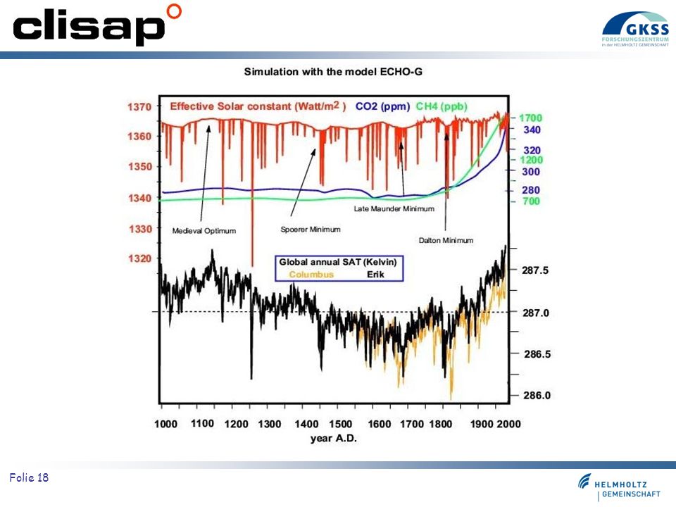
17. Forced Simulation 1000-2000 simulation Changing solar forcing and
time variable volcanic aerosol load;
greenhouse gases

19. Late Maunder Minimum 1675-1710 vs. 1550-1800 validation
Reconstruction from historical evidence, from Luterbacher et al.
Late Maunder Minimum
Model-based reconstuction vs

20. Global 1675-1710 temperature anomaly

21. Climate change simulations

23. Scenarios of what?
Climate = the statistics of weather, usually described by probability density functions, in particular by - their moments (e.g., mean, std deviation, covariances), - percentiles and return values, - spatial characteristics (e.g., EOFs), - temporal characteristics (autocovariance function, spectra)

24. Scenario building Construction of scenarios of emissions.
Construction of scenarios of concentrations of radiatively active substances in the atmosphere.
(Ok – not quite exact; aerosols …)
Simulation of climate as constrained by presence of radiatively active substances in the atmosphere (“prediction” of conditional statistics).

25. “SRES” Scenarios SRES = IPCC Special Report on Emissions Scenarios
A world of rapid economic growth and rapid
introduction of new and more efficient technology.
A very heterogeneous world with an emphasis on
family values and local traditions.
A world of “dematerialization” and introduction of
clean technologies.
A world with an emphasis on local solutions to
economic and environmental sustainability.
“ business as usual ” scenario (1992). A1 A2 B1 B2
IS92a
IPCC, 2001

26. Scenario building
Simulation with global models, which describe several compartments of the global earth system – relatively coarse spatial grid resolution (e.g., 200 km)
Simulation with regional models, often with only one or a few compartments (mostly atmosphere) – relatively high spatial grid resolution (e.g., 50 km)
Simulation with impact models – a large variety of different systems, e.g., storm surges or ocean waves.

27. Annual temperature changes [°C] (2071–2100) –(1961–1990)
Scenario A2
Annual temperature changes [°C]
(2071–2100) –(1961–1990)
Scenario B2
Danmarks Meteorologiske Institut

28. IPCC (2001) „regional development“ scenarios A2 and B2.
precipitation
Giorgi et al., 2001
Agreement among 7 out of a total of 9 simulations

29. Typical “global” atmospheric model grid resolution with corresponding land mask. T42 used in global models. (courtesy: Ole Bøssing-Christensen)

30. global model variance Spatial scales Insufficiently resolved
Well resolved
Spatial scales

31. Downscaling

32. Regional and local conditions – in the recent past and next century
Simulation with barotropic model of North Sea
Globale development (NCEP)
Tide gauge St. Pauli
Dynamical Downscaling CLM
Cooperation with a variety of governmental agencies and with a number of private companies
Empirical Downscaling

33. Typical regional atmospheric model grid resolutions with corresponding land masks km grid used in regional models (courtesy: Ole Bøssing-Christensen)

34. regional model variance Spatial scales Added value
Insufficiently resolved
Well resolved
Spatial scales
Added value

35. Concept of Dynamical Downscaling RCM Physiographic detail
3-d vector of state
Known large scale state
projection of full state on large-scale scale
Large-scale (spectral) nudging

36. Example Extreme Events (Wind & Waves)
2, 5, and 25-year return values with 90% confidence limits based on Monte Carlo simulations each.
(Weisse and Günther. 2006)

37. What is coastDat?
A set of model data of recent, ongoing and possible future coastal climate (hindcasts , reconstructions and scenarios for the future, e.g., )
Based on experiences and activities in a number of national and international projects (e.g. WASA, HIPOCAS, STOWASUS, PRUDENCE)
Presently contains atmospheric and oceanographic parameter (e.g. near-surface winds, pressure, temperature and humidity; upper air meteorological data such as geopotential height, cloud cover, temperature and humidity; oceanographic data such as sea states (wave heights, periods, directions, spectra) or water levels (tides and surges) and depth averaged currents, ocean temperatures)
Covers different geographical regions (presently mainly the North Sea and parts of the Northeast Atlantic; other areas such as the Baltic Sea, subarctic regions or E-Asia are to be included)
contact: Ralf Weisse 37

38. Some applications of Ship design Navigational safety
Offshore wind - Oils spill risk
Interpretation of measurements
Chronic Oil Pollution
Ocean Energy
Wave Energy Flux [kW/m]
Ocean Eneregy: Oberes Bild. zeigt den Wellenenergiefluss im langjaehrigen Mittel in Kilowatt/Meter senkrecht zur Wellenlaufrichtung. Normalerweise wird groesstes Potential in mittleren Breiten erwartet, die Deutsche Nordseekueste hat jedoch mit ca kw/m nur ein relativ geringes Potential (Bsp. 200 km Kuestenlinie x 10 kW/m = 2000 MW Leistung). Unteres Bild: Stroemung. Energiefluss in W/m2 Querschnittsflaeche (Rotor). Das skaliert im wesentlichen mit Stroemungsgeschwindigkeit hoch 3. Man sieht, dass das Potential raeumlich sehr begrenzt ist (z.B. List, Hoernum, Elbe, Jade) auf Fahrwasser, Rinnen und Seegaten (Nutzungskonflikte) und eher gering ist. Oft Argument: Wasser groessere Dichte, als Luft, deshalb Potential groesser als bei Wind. Das kann man mit folgenden Ueberlegungen relativieren: Potential proportional zu Dichte x Geschwindigkeit hoch 3 Dichte Wasser >> Dichte Luft (Faktor 1000), aber Geschwindigkeit Luft >> Geschwindigkeit Wasser (Faktor 10, 3. Potenz = Faktor 1000) und Wind steht grossflaechig zur Verfuegung, hohe Stroemungen (1 m/s) nur sehr lokal.
Currents Power [W/m2] 38

39. Scenarios for Northern Germany

40. A2 - CTL: changes in 99 % - iles of wind speed (6 hourly, DJF): west wind sector selected (247.5 to deg)
Scenarios for
HIRHAM
RCAO
Woth, personal communication

41. North German Climate Office@GKSS
An institution set up to enable communication between science and stakeholders
that is: making sure that science understands the questions and concerns of a variety of stakeholders
that is: making sure that the stakeholders understand the scientific assessments and their limits.
Typical stakeholders: Coastal defense, agriculture, off-shore activities (energy), tourism, water management, fisheries, urban planning

42. Online-Atlas „Klimawandel Norddeutschland“
Darstellung unterschiedlicher Größen zum Klimawandel in Norddeutschland für die Zeiträume , und
Darstellung der Differenz zu dem Kontrollzeitraum
Darstellung unterschiedlicher Treibhausgasszenarien (nach dem IPCC) gerechnet mit verschiedenen regionalen Modellen
norddeutscher-klimaatlas.de/ 42

43. Conclusions
Global climate modeling allows the representation of global, continental and sub-continental scales. Global models fail on the regional and local scale.
Global climates is varying because of both internal dynamics as well as external forcing.
Scenarios of future climate change hinge on the validity of economic scenarios.
Simulation of regional climate is a downscaling problem and not a boundary value problem.
Marine weather (winds, waves) have been successfully reconstructed for the years with a 1-hourly resolution.

44. Background information on this issue:
von Storch, H., S. Güss und M. Heimann, 1999: Das Klimasystem und seine Modellierung. Eine Einführung. Springer Verlag ISBN , 255 pp
von Storch, H., and G. Flöser (Eds.), 2001: Models in Environmental Research. Proceedings of the Second GKSS School on Environmental Research, Springer Verlag ISBN , 254 pp.
Müller, P., and H. von Storch, 2004: Computer Modelling in Atmospheric and Oceanic Sciences - Building Knowledge. Springer Verlag Berlin - Heidelberg - New York, 304pp, ISN X 44

45. http://coast.gkss.de/staff/storch hvonstorch@web.de
Weblog KLIMAZWIEBEL 45